2 Science and Systems Analysis
Jason Kelsey
As the words “science” and “systems” are part of the title of this book, it seems reasonable for us to examine them before we proceed any further. Why are they important enough to earn such prominent placement on the cover? In short, science and systems analysis provide a framework and tools that we will use extensively in our exploration of Earth’s natural systems. These concepts also are useful in the study of many subjects outside of the sciences. In other words, knowledge of them has broad, inherent value.
Key concepts
After reading Chapter 2, you should understand the following:
- The ways science is a distinctive way of knowing
- How evidence-based conclusions differ from those derived from opinions, values, and other subjective claims
- What can and cannot be assessed with science
- How the scientific method is used to objectively collect data
- Scientific conclusions, theories, and laws
- The sources and expression of measurement uncertainty
- The distinctions among accuracy, precision, and sensitivity
- How systems are defined and used to study many kinds of phenomena, including environmental processes
- The nature and importance of feedback in the functioning of systems
- How input-output analyses are important to environmental scientists
2.1. SCIENCE
2.1.1. Science is a distinctive way of knowing
Put simply, science is a way of knowing, one approach to a study of the universe (or, as scientists often say, the natural world). There are other ways of knowing, and science should not be held up as the only legitimate one. However, it is important to recognize the ways science is distinguished from those others and, critically, when it is the proper choice as a tool for analysis.
Our formal discussion of science will begin with a description of what it is not. First, although it is common for people to cite “scientific proof” when they attempt to make a convincing argument, science is not actually able to prove anything. Instead, it presents evidence and describes how certain we are about conclusions and ideas. Degrees of certainty are vital to the practice and understanding of science, as we will see in more detail shortly. Second, science cannot be used to assess subjective ideas or evaluate notions about what is good or bad and right or wrong. It is not values or faith based and cannot (and should not!) be used to try to somehow answer questions about the meaning of life, the quality of a musical composition, the morality of cutting down trees, or even the existence of God. It is not the right tool to answer aesthetics questions such as “do these pants look nice on me?” or “is this painting good?”. We also should not ask scientists to comment on environmental questions such as whether an endangered species or ecosystem has a right to exist, rather, we can draw upon science to predict the likely consequences to natural systems if a particular organism disappears and use it to inform our decision making. In other words, although science is very powerful, it is also limited.
What then, is science? What can it do? In short, science is an evidence-based approach used to answer testable questions. Its fundamental goal is to reveal generalizations—the rules, if you will—governing the universe. It is distinguished from other ways of knowing and evaluation by some important characteristics.
2.1.2. Science is objective
Scientists seek to increase our understanding of the natural world. They design experiments and record observations but do not interfere with the way experiments unfold. Crucially, personal bias, values, or preconceived notions about what should be true, what the answer to questions of interest ought to be, are irrelevant. Ideally, such emotional involvement is completely absent. Since science is carried out by humans, subjective judgments can affect the way real-world science is conducted. Accordingly, potential conflicts of interest or bias should be acknowledged and described in all scientific studies.
2.1.3. Science requires evidence
Unless data can be objectively collected, science is not the proper tool to study a particular phenomenon or question. In other words, explanations that require inference, intuition, faith, or indirect connections between cause and effect are not in the realm of science (see Correlation vs. Causation, below, for more about the relationship between cause and effect). Science is only appropriate if an idea can be tested through observation, that is, some kind of experiment that allows for the collection of empirical data is required. Now, experiments vary widely in their nature and ability to mimic reality, but they are still a necessary part of scientific inquiry. Chemists, physicists, geologists, biologists, and ecologists collect data under vastly different circumstances using experiments and tools that are unique to their disciplines. Some primarily observe existing natural systems, whereas others conduct controlled experiments inside laboratories. Some scientists rely entirely on computer models. In all cases, though, they use objective methods and what is commonly referred to as the scientific method to gather evidence. We will consider more about what constitutes an experiment and how experimentation is a part of the scientific method shortly.
2.1.4. Science uses both inductive and deductive reasoning
As we learned above, science is used to study the natural world, but there are multiple ways to carry out such inquiries. Scientists may examine representative cases—they collect individual data points—and then attempt to establish a plausible and widely applicable explanation for what has been observed. In other words, science often employs inductive reasoning: it uses specific observations to establish new generations. Imagine a very simple example in which we study the behavior of falling objects. To accomplish this, we could set up an experiment in which we throw various things out of a seventh-floor window and record what happens. We might begin with a computer, and then follow with a chair, a piece of chalk, a coffee mug, and a melon. Assume we drop twenty objects and they all smash pleasingly on the pavement below. After a while we would likely tire of this exercise (or simply run out of objects to hurl) and decide that we have enough data to try to establish a general rule about all falling objects based on our limited number of specific observations. We could then develop ideas about gravity and so forth that we would assume are broadly applicable. Note that the degree to which the new generalization describes every possible case will depend on how representative our specific observations are. In other words, if the rule we establish is to be valid, the objects we drop from the seventh floor need to behave like anything else that falls to the ground. If we chose live birds, helium-filled balloons, soap bubbles, or flat sheets of paper, our observations would not apply to all relevant situations and could lead to potentially disastrous conclusions. We will come back to this and other potential problems affecting experiments when we discuss uncertainty, below. On the other hand, deductive reasoning is the opposite of inductive reasoning in that it is used to test if specific cases follow pre-determined rules (that is, it progresses from the general to the specific). For example, the rules of geometry tell us if a given unknown shape is a triangle, square, circle, etc. Scientists could also use deductive reasoning to test whether a hypothesis or prediction is supported by experimental evidence, that is, specific cases that are analyzed in an experiment. In this latter instance, we assume the generalizations are true until shown to be otherwise.
2.1.5. How it is done: the scientific method
The scientific method is a systematic approach that has been used for centuries in countless studies of the natural world. Classically and formally, it consists of several stages, although it is worth noting that the scientific method as described here represents an idealized version of the way science is conducted. All experiments do not necessarily follow each and every step in the order shown, but they broadly use the approach outlined here.
1. Observation
A scientist notices a phenomenon and decides to study (and, they hope, explain) it. Typically, this is a moment when a question that starts with “how does…” or “why does…” or “what is…” is formulated. It can be a question about anything, but it is likely something that seems important or interesting to the scientist asking it.
2. Hypothesis
The scientist develops a plausible answer to the question posed in step 1, above. In other words, this is the step in which a hypothesis is formulated. Put simply, a hypothesis is a proposed explanation for the observed phenomenon of interest. People sometimes refer to this as a “guess”, although such a characterization is not entirely appropriate. Usually, a hypothesis is put forth only after careful thought and review of what is currently known about related phenomena.
3. Experiment
Experiments are designed and conducted to test the validity of the hypothesis. As we saw above, there are many different types of experiments, but they all involve observation and data collection. Scientists examine data and draw a conclusion based on them. The conclusion reached is an answer to the question posed in step 1. At this stage, the answer suggested by the experimental data is compared to the hypothesis, and the hypothesis is either supported or refuted. Remember that science cannot provide absolute proof that anything is true, instead, it can make a case that a proposed explanation is appropriate by supporting a hypothesis multiple times under differing conditions (interestingly, when experiments do not support a hypothesis, we typically say something like “the hypothesis is disproven”). For example, one might measure how the amount of sunlight received can influence the growth of a certain plant. A scientist would start out with a hypothesis that is something like “plant growth will depend on sunlight received; both insufficient and excess light will adversely affect the height a plant reaches within two months.” The experiment would involve groups of plants exposed to different amounts of sunlight (say, nine groups ranging from complete darkness to continuous light, with ten plants in each group—i.e., light is the variable we assess). The plants would otherwise be treated identically (same amount of water, soil, etc.). The scientist would measure the heights of the plants each week for two months. At the end of the experiment, a conclusion about the relationship between light received and plant height would be formulated. The validity of the initial hypothesis would also be evaluated given the data collected (Table 2.1). Note that an important part of our conclusion is that different amounts of sunlight caused the observed differences in growth; the two were not simply correlated (for more, see Correlation vs. Causation, below).
Table 2.1. Effect of sunlight on plant height
| Light (hours) | Height (cm) |
|---|---|
| 0 | 0.0 |
| 3 | 4.1 |
| 6 | 7.3 |
| 9 | 15.2 |
| 12 | 17.8 |
| 15 | 21.6 |
| 18 | 18.5 |
| 21 | 14.6 |
| 24 | 9.2 |
4. Retest or refine a hypothesis
If the initial hypothesis is supported by the data collected, the experiment should be conducted again. An experiment must be repeated multiple times, and data must be compiled from many studies before scientists can begin to make generalizations about the phenomenon of interest. In the plant experiment imagined in step 3 we could analyze the data and conclude that there is an optimal amount of light exposure for plant growth (15 hours a day in this case, as shown in Table 2.1). In other words, our hypothesis seemed to be valid. The next step for us could be to carry out the whole experiment again and compare the findings from the two studies. We might decide to repeat this process many times. If, however, the hypothesis is refuted, or only partially supported, we would have to revise it.
5. Communication and review of results
Once scientists have repeated an experiment and reached some conclusions about the phenomena under investigation, they must then communicate that information to the scientific community. Such sharing enables other scientists to scrutinize and repeat the experiments on their own to independently test the conclusions drawn from them. Results can be shared informally—among colleagues at the same or different research institutions—or formally, through a published paper or oral presentation. An important part of formal communication is what is known as the peer review process. Researchers wishing to publish in a scientific journal, for example, generally submit their manuscript to an editor. Scientists with the appropriate education and experience then review the submission to determine if it should be accepted for publication (generally, they insist on a number of revisions to the manuscript in any case) or rejected. Oral presentations are vetted to varying degrees, but a scientist presenting data to an audience will be subjected to questions and expected to justify and defend the work most of the time. Science is therefore scrutinized and challenged, requiring researchers to objectively and carefully study the natural world. Put another way, whether as formal reviewers or simply readers of scientific journals, scientists are expected to be skeptical of conclusions presented to them—they should not accept any new idea until they have studied and challenged it thoroughly. Of course, all this rigorous checking and review mean that our understanding of the universe advances gradually. Contrary to the way they are often portrayed in popular culture, scientists very rarely exclaim “Eureka!” or the like. Sudden breakthroughs and discoveries are the exception, not the rule.
2.1.6. Correlation and causation are not the same
When we are conducting experiments to test the effect of some variable on the behavior of objects or organisms it is important to distinguish between correlation and causation. Correlation refers to the way two events occur at the same time but suggests nothing about the ways one of the events influences the other. Causation implies that the two events under investigation are connected and that one led directly to the other. Although it can be tempting to assume a stressor brought about observed changes just because two events are simultaneous (or sequential), science strives to actually establish a link between cause and effect. Imagine we decided to study the relationship between the presence of a cigarette lighter in one’s pants pocket and the development of lung cancer. The data would show that cancer occurs in people who carry lighters more often than in those who do not (see Figure 2.1).
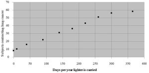
We can see that lung cancer is correlated with the carrying of a lighter. It is likely not surprising to you, however, that lung cancer is not caused by the presence of a cigarette lighter, rather, lung cancer is directly linked to cigarette smoking (which is tied to carrying a lighter). A less fanciful example can be seen in the debate about the relationship between childhood vaccinations and autism. Although some children start to exhibit signs of autism shortly after receiving the MMR vaccination, there is no evidence that the vaccine brings it on. In fact, numerous studies conducted to test whether or not vaccines cause autism have repeatedly shown that although sometimes correlated in time, there is no mechanistic link between the two. See Box 2.1 for more on autism and vaccination.
Box 2.1. Correlation is not causation: the case of vaccines
Whether phenomena are linked by causation or only correlation is an important consideration, as a misunderstanding could lead to the misallocation of resources to treat a neurological difference such as autism. In other words: because of efforts by a small yet vocal group of people who are adamant that childhood vaccination is responsible for autism, money, energy, and time are diverted away from research that could reveal its actual cause. Furthermore, and arguably more problematic, some people who think autism is brought about by vaccination refuse to have their children immunized against a wide range of preventable illnesses. The result can be a public-health crisis. For example, an outbreak of measles in some California public schools (and Disney theme parks) in early 2015 was driven by low vaccination rates. Many of the parents of unvaccinated children decided against inoculation because they believed it posed health risks. Objective interpretation of data, though, has led all but a few scientists and physicians to conclude that the risk associated with contracting measles is far higher than that of receiving the MMR vaccine. Review Box 1.2 for more about cost-benefit analysis.
2.1.7. Experimental vs. observational science
In addition to helping uncover the rules of the universe, the scientific method can be used to classify and identify components of the natural world. These two uses of science are referred to as experimental and observational, respectively.
Experimental science
Here, scientists assess the effects of stimuli on test subjects (objects, organisms, etc.). The experiment described above involving the relationship between light received and plant growth is a good example of experimental science. Note that the responses of test subjects must be compared to control subjects, those that go untreated. A group of animals that does not receive an experimental drug, say, but otherwise is identical to those that do, would be a good example of the use of controls. As we have seen, new generalizations about the ways the universe functions are developed with experimental science.
Observational science
In this case, scientists collect information about a test subject at a moment in time. The effects of changing conditions are NOT assessed in observational science, neither are the subjects influenced by or exposed to stressors during these types of studies. Observational science can be applied to many situations. For example, we could study the long-term effects of smoking on human health by surveying a group of people to assess any connections between smoking (how much per day, number of years a person smoked, etc.) and the occurrence of diseases such as cancer and heart attack. Remember, the test subjects would not be given cigarettes and then observed for years afterwards, instead, we would study their health status today in light of the smoking they did previously (you might imagine that such a study is fraught with difficulty and uncertainty, in part because we must rely on test subjects to report their smoking habits). Observational science could also be used to determine public opinion (e.g., people are polled about how they will vote), or to classify birds, rocks, and other objects into appropriate groups. In all cases, test subjects must be evaluated (through questioning or other means) in an objective way and should not be manipulated or influenced such that their present condition is altered.
2.1.8. Conclusions, theories, laws: just how confident are we?
As we have seen, experimentation leads to notions about the rules governing the universe. You should recognize that our understanding evolves as more and more research is conducted, and our level of confidence about this understanding evolves similarly. For clarity, scientists use three basic terms to indicate the level of certainty associated with a scientific idea. The first, conclusion, is the most tentative of the three. It is derived from the results of a small number of experiments and is expected to change as additional data are collected. Conclusions can be applied only narrowly. With more time and study, and repeated challenges and revisions, a conclusion can be elevated to the second level, that of theory. Theories are widely accepted explanations of important phenomena. Two of the most well-known theories are that of plate tectonics and biological evolution (Chapters 3 and 5, respectively). Both have been developed, studied, and scrutinized by many generations of scientists, are supported by a lot of data, and are thought by most to plausibly describe the development of Earth’s surface and its life, respectively. These and other theories have withstood over a century (or more) of close examination and attempts to refute them and yet continue to be supported by data. Despite their longevity and apparent validity, scientists do not stop studying and revising theories, however. In fact, theories could be shown to be invalid, or at least change, with enough data. Finally, after even more time and many more experiments designed to test a theory, some ideas become so well entrenched that they are elevated to the highest level, that of scientific law. Because the criteria that must be met are so rigorous, relatively few theories have become laws. The laws of thermodynamics (Chapter 4) and gravity are among the important examples of the types of generalizations thought to be worthy of this categorization. Few think they will be refuted, although scientists must always allow for the possibility that our understanding of even these most foundational principles could change with continued study.
2.1.9. Scientific measurement and uncertainty
Measurements in experimentation
Tools, or instruments, are used in science to quantify (assign a number to) properties including length, temperature, mass, volume, and chemical composition of the objects they study. For instance, one could respond to the question “How long is this tree branch?” with an answer like “The branch is 3.2 meters (m) in length.” Notice that the length is expressed with both a number and unit. The unit given is universally accepted and recognized by all (or nearly all) scientists. For the length of interest in this case, the appropriate tool would likely be a meter stick. As we will see shortly, a meter stick is not the best device with which to measure the length of all objects (see Accuracy, Precision, and Sensitivity, below). Thermometers, balances (essentially the same as scales), and other instruments assess various properties. Although a range of tools can be used to quantify many different characteristics, all measurements have something important in common: they represent approximations of the actual values of interest. In other words, every measurement has some amount of uncertainty associated with it. Even the most experienced scientist working under the best circumstances must still contend with the reality of scientific uncertainty.
Uncertainty happens!
Imagine that you are hosting a dinner party and serving wine to your guests out of a glass carafe (you secretly combined the remains of several opened bottles of wine you had lying around, some of which are less than spectacular). Before pouring the last round, you want to determine the volume of wine remaining. In the kitchen you transfer the wine to a cup measure and conclude that there are a little under 4 cups (945 mL) in the pitcher. You are pretty sure this amount is sufficient to just fill the glasses, but because the cup measure is not fancy enough to use in front of your guests, you dump the wine back into the carafe and hurry back into the dining room. To your surprise (and embarrassment), you are not able to top off all the glasses evenly, and the last person in line for a refill gets visibly less wine—by a fair amount—than everybody else. Somehow, it seems you do not have the 945 mL of wine you measured in the kitchen. After your guests leave, you decide to figure out what happened and recreate the awkward situation from earlier in the evening. You add 945 mL of water (your guests drank the last of your wine) to the cup measure and then use it to fill the five glasses still sitting at the table. Remarkably, this time there is sufficient water to fill the glasses adequately. You are puzzled and want to pursue this minor mystery. So, you repeat the steps you took, noting that there are different amounts of water left to fill the final glass each of the six times you carry out the test. As a next step you choose to dump the water back into the cup measure to determine the total amount present in the five glasses after they have been filled. You write down the volume left after each trial and come up with the following six numbers: 940, 938, 937, 935, 929, and 917 (all mL). How could this be? What happened? Why do you get six different numbers? The answer to these questions is linked to experimental error and scientific uncertainty, and we will return to it shortly.
Experimental errors
Outside of science, the word “error” generally refers to a mistake or an accident. If you drop the glass pitcher of wine (from our scenario, above) and it shatters on the floor, you might use the word to describe your action (with or without other, less refined, words added for emphasis). In a more scientifically relevant example, if you intend to determine the height of something but instead measure its width, you will have made a mistake. Importantly, that mistake can be corrected if you redo the work. However, the word means something quite different when used in the context of measurement. Put simply, experimental error is defined as the difference between the measured value of a property and the actual value of that property. For example, if the temperature of a liquid is 25.6 °C but you measure it as 25.1 °C, you are off by 0.5 °C, that is, your error is 0.5 °C. Unlike the mistakes described above (dropping the glass pitcher, etc.), not all experimental errors can be corrected simply by repetition. In fact, although they can be minimized, they cannot be eliminated—errors are an inherent part of every measurement and must be quantified and reported in any experiment.
Systematic errors (= determinate errors)
These affect accuracy, how close a reading is to the actual value (see the section below, Accuracy, Precision, and Sensitivity, for more information). Because of these types of errors, every one of the readings of the same phenomenon is wrong in the same direction: they are all either higher than or lower than the actual value. Systematic errors tend to arise from faulty or uncalibrated instruments or human error (more about calibration is described below in the section Accuracy, Precision, and Sensitivity). For example, imagine you are using a cloth tape measure to determine the length of a snake you found under your porch. Unfortunately, since it has been stretched out from years of heavy use (yes, you live in a snake-filled swamp), it consistently yields readings that are too short (i.e., although the tape “says” it is measuring something at 1 m, the object is actually 0.9 m long). You might take twenty measurements of the snake, but each will be wrong—too long—because the instrument you have is faulty. Using a consistently bad technique to make a measurement will also generate systematic errors (e.g., a scientist might not know how to properly read an instrument). Importantly, no matter how many times you repeat a measurement, it will remain inaccurate. Strategies that do work to reduce systematic errors include calibration of instruments and training of scientists doing the measuring.
Random errors (= indeterminate errors)
These errors affect precision, how well multiple readings of the same phenomenon agree with each other (again, see Accuracy, Precision, and Sensitivity for more information). Unlike systematic errors, random errors lead to a group of measurements that is off in both directions: some will be above and some below the actual value. Random errors arise from variables that are difficult or impossible to control. Consider how a hypothetical experiment conducted in an outdoor field to assess the effects of fertilizer amount on plant growth will be affected by weather. Among other problems, each day, conditions such as temperature, sun exposure, and moisture will change. It is possible that differences in growth are linked to climatic factors and not fertilizer availability at all. Variation in responses among different test organisms, termed biological variability, is another common source of these types of error. For example, one laboratory rat will likely respond differently to the same dose of a drug undergoing testing than will a second rat. Scientists can also introduce random errors by the way they take and read measurements. Imagine you are trying to determine the volume of water in a glass container. You read the markings on the wall of the container (called graduations) and notice that the top of the solvent lies between the 17.5 and 17.6 milliliter (mL) marks (see Figure 2.2).
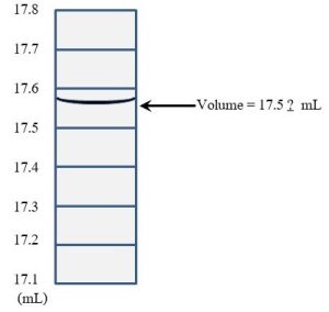
Generally, researchers will estimate the last digit using interpolation. In our case, you would look at the liquid and make a reasonable guess about what number should go in the 100ths place. After staring at it for a while, you might decide that 17.56 is the best answer. A different person might say 17.58, a third 17.54, and so forth. No matter what you do, there is some subjectivity associated with this measurement, and, as a result, such a data set will contain points that are clustered both above and below the actual answer. Unlike systematic errors, repetition can reduce the size of the random error. If one takes 5, 10, or even 100 measurements of the same phenomenon, error will be reduced (which can be demonstrated using the tools of statistics, something that is beyond the scope of this text). In any case, a single measurement would be considered insufficient to draw any useful conclusions—more data points are always better than fewer. Taking steps to minimize variables can also reduce these types of errors. In the field experiment suggested above, we might control weather conditions by moving all the plants to a greenhouse. In this way, we can isolate the variable we would like to study, the effect of different amounts of fertilizer on plant growth, and keep everything else constant (i.e., the same for all plants). In drug testing, the use of large numbers of animals that are as identical to each other as possible and the development of standardized procedures will reduce random errors as well (see Chapter 15 for more about drug testing).
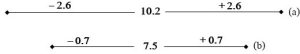
Determining and reporting experimental errors. A well-designed experiment includes multiple readings of the same phenomenon. In other words, we would not make any conclusions about plant growth (our experiment above) by looking at a single plant. We would instead treat several plants in the same way and try to determine some representative answer based on observations of the group. Remember that biological variability will cause individual organisms, even those that are very closely related, to respond differently to the same stressors. So, we will likely get multiple responses, perhaps as many as ten, in the group of ten plants provided with the same amount of nutrients. How do we resolve one question with ten different answers? Although there are several ways to handle such a situation, a commonly used strategy is to calculate the mean (i.e., average) and standard deviation of each group to express an answer. In somewhat oversimplified (yet reasonable) terms, standard deviation represents our level of uncertainty, or, put another way, the range within which the actual answer is likely to be found, and the mean is used to suggest the most likely answer in that range (i.e., it is an appropriate representation of the actual answer). Consider two data sets (given as mean ± standard deviation): 10.2 ± 2.6 and 7.5 ± 0.7. For the first, we can approximate the range as 7.6 – 12.8 and for the second 6.8 – 8.2. Importantly, a bigger standard deviation indicates a larger amount of error and lower confidence in the data, which may be more easily visualized graphically (Figure 2.3).
Progress despite errors. If every measurement is only an approximation, how do we ever learn anything about the natural world? How can scientists retain their sanity if they are constantly dealing with error? Might it be preferable to just close down their laboratories and open up ice cream shops? It turns out that, despite uncertainty, there are ways to interpret the ranges indicated by means and standard deviations to draw conclusions and keep science moving forward. The details of the mathematics involved in analyzing data are not the point of this textbook, but in short, it is possible to determine relationships among groups receiving different treatments (i.e., exposed to different conditions) in an experiment. Through the mathematical equivalent of comparing the ranges of the groups and looking for likely overlaps, a scientist can determine the effects of a changing variable on the subject under study. A fundamental yet critical concern is whether groups of test subjects receiving different treatments are different from each other, that is, whether the variable of interest has a real effect that cannot be explained away because of uncertainty. Recall the experiment in which we studied the effect of different amounts of fertilizer on the growth of plants. Among other things, we want to determine if the groups are different from each other—if and how nutrient availability affects growth. To simplify our discussion, we could compare the size of the plants at only the highest and lowest nutrient conditions. The measured masses from the ten different plants in each group are presented in Table 2.2.
Table 2.2. Effect of fertilizer on plant growth. “±” denotes “plus or minus”, how far the error term goes above and below the mean.
| Mass of Plant at Harvest (grams) | |
| Low Fertilizer | High Fertilizer |
| 35.2 | 44.4 |
| 34.3 | 47.1 |
| 29.1 | 48.3 |
| 27.5 | 50.2 |
| 37.2 | 39.7 |
| 33.0 | 42.1 |
| 32.6 | 43.5 |
| 30.9 | 46.7 |
| 26.4 | 41.6 |
| 38.8 | 49.2 |
| Mean | |
| 32.5 | 45.3 |
| Error | |
| [latex]\pm4.1[/latex] | [latex]\pm3.5[/latex] |
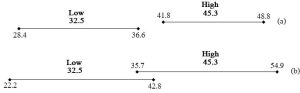
Now, it might seem odd to even wonder such a thing, but we want to know if the two groups are different from each other. Although 45.3 is surely a higher number than 32.5, differences in the amount of growth of individual plants receiving the same amount of fertilizer complicate a seemingly simple comparison and leave open the possibility that the two numbers need to be thought of as the same. There are many responses that we must consider when we try to make our conclusion: plants receiving less fertilizer produced between 28.4 and 36.6 g of tissue whereas plants receiving more produced between 41.8 and 48.8 g. Again, keeping things fairly simple, we can scrutinize the ranges to determine how likely it is that 45.3 really is higher than 32.5. As before, we could use formal statistics to confirm our conclusion, but a visual inspection reveals what the math would tell us, namely, that there is no overlap between the two groups (see Figure 2.4a). Even if the low-fertilizer growth is as high is it could possibly be (36.6 g), it is still less than the smallest amount of growth under high-fertilizer conditions (41.8 g). We can be reasonably confident, therefore, that the two groups are different and that plants grow better with the higher level of fertilizer. However, what if our error terms were substantially larger, say 10.3 for the low group and 9.6 for the high group? Our ranges would become 22.2 to 42.8 and 35.7 to 54.9 for the two groups, respectively. As unsatisfying and perhaps illogical as it might seem, we would be forced to conclude that 45.3 and 32.5 are not necessarily different from each other—it is possible, given uncertainty, that growth under low-fertilizer conditions is the same as or even high than that under high-fertilizer conditions. In this case we could either report those findings (i.e., amount of fertilizer does not affect growth) or, in all likelihood, redesign and repeat the experiment to try to reduce uncertainty (see above for ways to shrink the error). Figure 2.4b shows the overlapping ranges for our second case.
The inclusion of an error term is necessary for the proper understanding of data both in- and outside of the sciences. You likely have seen how public opinion polls designed to predict the outcome of upcoming elections tend to provide an indication of uncertainty when they are reported. In a hypothetical race for U.S. President, one candidate might be polling at 47% and the other at 44% with a margin of error of ± 5%. Numerous factors could account for the uncertainty, including the facts that only a small subset of people is used to represent the entire voting population and poll questions could be misinterpreted by respondents. In any case, because the ranges overlap, the most reasonable conclusion is the race is currently a tie, or “too close to call.” Of course the answer revealed on election day can act as a kind of check on the quality of the polling—how well voters’ behavior was predicted by today’s survey can inform the reliability of future polls done by a particular organization. Put another way, election results can be used to calibrate a poll (more about calibration is described below). We can only evaluate results of experiments, and come to whatever conclusions they suggest, if uncertainty is rigorously calculated and described.
Accuracy, Precision, and Sensitivity
Although they are sometimes used interchangeably in casual settings, these terms have three distinct and important meanings to scientists.
Accuracy. This term refers to correctness, how close a measurement is to the actual value of the property we are assessing. So, if we determine the mass of an object to be 10.3 g when the true value is 10.6 g, we are inaccurate by 0.3 g. It is a relatively simple matter to determine just how wrong we are if we happen to know the true mass of the object in question. But what if we do not know the actual value? How then can we judge accuracy? Remember the example of the polling data from above. We can try to predict the outcome of an election by sampling the opinions of voters, but our answer will have some level of uncertainty associated with it and will likely be wrong by some amount. Just how good our polling methods are can be tested by comparing our prediction to what happened in the election. We have the luxury to learn the right answer to the question. When the actual value is not available to us (which generally is the case in science) we instead rely on calibration, that is, we use an object with a known value for the property in question (mass, length, volume, etc.) to test our instrument. When determining the mass of an object, for example, we ought to consider whether the balance we are using is working correctly. To be flip about it, does the balance know what it is doing? Does it have any idea what a gram even feels like? To answer these questions we can acquire a calibration weight, an object with a known mass, and measure it on our balance. If the object we know to be 1.0000 g is assigned a mass of 0.9986 g on our balance, we need to reset, or calibrate, the instrument with the 1.0000-g mass to improve the accuracy of future measurements. The same must be done regularly with meter sticks (length), graduated cylinders (volume), and other laboratory instruments. See Box 2.2 for more on calibration.
Box 2.2. How do we know what 1 g really is?
Before you attempt to use a balance, you should check the instrument with a carefully manufactured object of a known mass. If the mass reported by the instrument to be used is either more or less than that of the test weight, then you know that the balance is wrong, and you must calibrate before proceeding. We might think of this as telling the balance what the right answer is—or the standard against which it should compare—before we try to measure an unknown. But, what about that expensive calibration weight we purchased? How do we know that its mass is correct? The simple answer to this question may surprise you: there is an actual object stored at the International Bureau of Weights and Measures (near Paris, France) which, by international agreement, is considered to be the prototype of the kilogram (1000 g). All balances are ultimately compared to and calibrated with that universally accepted standard mass. Since the object is kept under glass inside a secure vault and only taken out occasionally, it is obviously not used directly. Copies of it, and copies of those copies (and so forth) are used to calibrate the world’s balances. The standard unit for length was similarly based on a single prototype, the meter, until the 1980s. Since then, a different way to define the meter has been used, although the idea of a universally accepted standard persists for it and other units.
Precision. This term refers to how well separate measurements of the same object (termed replicate measurements, or replicates) agree with each other. In other words, if you measure the volume of a liquid multiple times, how similar to each other are your replicates? Imagine one experiment in which we test the temperature of a liquid four times to yield the answers 35, 41, 29, and 45 °C, and in a second experiment we end up with 34, 36, 32, and 30 °C. As we saw previously when considering the effect of fertilizer on plant growth, there is a range of answers here. We could quantify our precision and our level of uncertainty using the tools of statistics, but in simple terms an examination of the two data sets reveals that there is a larger range (i.e., lower precision) in the first experiment relative to that in the second experiment. Like accuracy, precision is a critical property—but the two terms refer to very different considerations. In fact, as explored in Box 2.3, a set of data could be very precise yet still inaccurate.
Box 2.3. Accuracy vs. Precision, OR: close only counts in horseshoes and hand grenades….what about science???
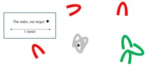
Just because you can get nearly the same number each of the dozen times you measure something, you should not assume your answer is accurate. You might generate a data set of readings that are tightly clustered together and record a mean with a small error term. Unfortunately, every one of the readings will be wrong, perhaps by a lot, if your balance has not been properly calibrated. We can use the somewhat old-fashioned lawn game known as Horseshoes to think a bit more about the distinction between accuracy and precision. Keeping things simple, in Horseshoes one throws an object—that’s right, a horseshoe—12 meters toward a vertical stake in the ground. If the horseshoe completely encircles the stake, the shot is called a ringer and 3 points are awarded. A throw that is not a ringer but lands within 15 centimeters (6 inches) of the stake is close enough to score 1 point. So, how are all these rules related to accuracy and precision? The highest-scoring and most-difficult shot, a ringer, can be equated with the right answer, or high accuracy. A less accurate shot is worth only 1 point. Now, it is possible that all the horseshoes you throw in an inning land close to or even on top of each other but still far from your intended target. Clearly you have made consistent throws if the shoes land together, but you still get 0 points if they sit 2 meters from the stake. In this case, you are both beautifully precise and horribly inaccurate (see Figure 2.5)! Although repeatability is often thought to be confirmation of correctness, you should be cautious and remember that precision and accuracy are not the same things.
Sensitivity. This final term is generally applied to the instrument used to make a measurement more than the data themselves, and, although it is distinct from both accuracy and precision, it can influence those two other properties. Simply put, sensitivity refers to the smallest measurement an instrument can make, or sometimes we say it is the minimum change an instrument can detect. The sensitivity of an instrument is a crucial consideration when one is making a measurement. For example, if you wanted to determine the size of a bacterium, a meter stick would not be the right tool to use. If you consider that bacterial cells are about 1 millionth the length of a meter stick (on the order of 0.000001 m, or 1 micron, long) the problem should become immediately clear. If you were somehow able to see a single bacterium lined up next to a meter stick (a significant challenge since bacteria are microscopic—consult Figure 2.6), you would notice that the cell is about a thousand times smaller than the smallest unit marked on the stick (millimeters, mm, or 0.001 m).
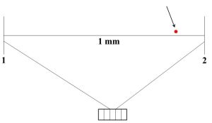
Even if it is perfectly calibrated, the best answer you can get with a meter stick is something unhelpful like “bacteria are a lot smaller than 1 mm”. The tool is clearly not sensitive enough to determine the length of a very small object. Similarly, it would be foolish to try to measure something with a mass of 0.0045 g using a balance that cannot detect changes smaller than 0.00 g. The balance would continue to read 0.00 before and after the object was placed on it. Keep in mind that, although accuracy and precision are not the same as sensitivity, they can still be adversely affected if an instrument does not measure small enough quantities. As you might imagine, it would be very difficult to determine the true value of the length of the bacterium we mentioned above with a meter stick. Getting replicate answers to agree with each other would also be nearly impossible under these circumstances.
Uncertainty happens, revisited
Now that we have considered sources of error and uncertainty, we are ready to return to the problem of insufficient wine at our dinner party. You will recall that, when we conducted our experiment to track down an explanation, we ended up with different amounts of water each of the six times we measured. How could this be? Well, many potential sources of error exist, including: the measuring cup might not have been properly calibrated, we could have read the volume from a different angle each time (leading to the different answers), and we did not account for water spillage during transfers back and forth (note that the volume left in the glass declined after each replicate, 940, 938, 937, 935, 929, 917 mL). Errors associated with the dinner party itself, such as our rush to get back to the dining room and our assumption about how much wine was required to fill the glasses, could have compounded the problem. Of course, the addition of alcohol into our bloodstream should not be discounted either. Other systematic and random errors surely could have affected the outcome in our situation. In short, even a problem as simple as pouring wine into multiple glasses is fraught with uncertainty. Imagine how many potential errors can affect more complicated environmental experiments! As we progress through this textbook, we will identify and manage sources of uncertainty yet still make reasonable conclusions about the natural world. This is the way of science.
What is the point of all this? What good is science anyway?
As we know, experiments are designed to objectively collect data. But to what end is science conducted? Does science serve any useful purposes? Although scientists tend to be drawn to their fields because they find them fascinating and simply enjoy learning how the world works, science is used extensively to address most of the practical questions important to society as well. Medicine, agriculture, nutrition, food safety, development of new materials, construction, cosmetics, pharmaceuticals, power generation, drinking water availability, air pollution, and waste management are but a sampling of the fields and products that depend on scientific inquiry. In fact, it is difficult to name many areas of modern life that are not directly informed and improved by science.
Before we leave our introduction to science, we must address one final and critical question, namely, who decides what should be studied? The answer to that question is tightly linked to another important, albeit somewhat crass, one: who pays for scientific research? Conducting science can be very expensive, and there is a finite amount of money available to do so. Much, but not all, of the funding for research is provided by government programs that tend to reflect the values and needs of society. So that means scientists must apply for money to support their work. Since the process associated with securing funding is generally extremely competitive, the questions to be asked, as well as the design of the experiments proposed to answer them, must be very well thought out and deemed relevant to society before funding is granted. Like the peer-review process for potential scientific papers described above, grant proposals undergo intense scrutiny by experts in the appropriate field before money is released. It is fair to say that there are many more losers than winners when it comes to competitive grant writing.
2.2. SYSTEMS ANALYSIS
Like the scientific method, systems analysis will serve us often and well during our exploration of Earth’s environments. In addition, you will soon see that the tools we learn here are helpful in the studies of many subjects, events, and processes far beyond environmental science.
2.2.1. A whole greater than the sum: the system definition
In very simple and general terms, an entity can be classified as a system if it meets certain criteria.
It is made up of component parts
These subunits are connected to each other somehow, affect each other, and broadly speaking, work together. The old expression “the whole is greater than the sum of the parts” is apt here because, through their connections and interdependence, the combined pieces can accomplish outcomes that are different than would be possible if they all worked on their own.
It can be distinguished from its surroundings
A system has characteristics and a discrete identity that set it apart in obvious ways from other entities. Since some systems are embedded within or firmly attached to other systems, this separation may be only conceptual, not physical. For example, the human digestive system is an entity in its own right, but clearly it cannot easily be disconnected and taken away from the other systems in the body without some unfortunate results for the person involved. A single human is itself a larger system that is physically and obviously distinct from other systems.
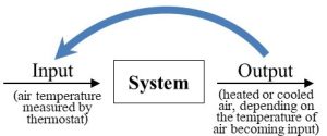
It receives inputs and produces outputs
Many kinds of factors (materials, energy, etc.) can enter a system and undergo processing by it. Those factors can be released by the system unchanged relative to the form they took when they entered, or they can be altered inside the system and exit as a part of new products. Figure 2.7 is a generalized way to visualize any system, including the relationship between inputs and outputs.
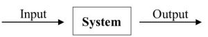
This model will appear throughout this book as it is an appropriate, not to mention very useful, way to help understand many environmental processes. Keep in mind that what a system produces is a function of what it receives: if inputs change, outputs will change as well. In other words, systems are responsive. We will consider some of the inputs and outputs that affect and are affected by systems shortly.
It interacts with other systems
Although systems can be defined as separate from their surroundings, rarely is a system completely isolated from all others. In fact, systems generally affect each other, and we categorize them based on the ways they interact. A system is closed with respect to a particular factor if it does not exchange that factor with other systems and open with respect to any factors it does exchange. Note that a system can be closed with respect to one factor and open with respect to others, so it is not correct to simply refer to a system as either “open” or “closed”—we should specify which factors are shared and which are not. Earth, for example, is closed with respect to materials and open with respect to energy (Chapter 1).
Size is irrelevant
They are made of component parts, but systems can range in size from microscopic to as big as the universe.
Many familiar phenomena and objects lend themselves to systems analysis
If you recall our basic definition from the beginning of this section, you will start to notice systems all around you. Before we proceed any further with our general discussion, it might be helpful to consider a few specific entities that are good examples of systems.
A person. An individual human being can be viewed through the lens of system analysis because it meets the basic criteria. First, it is made up of components that work together. The circulatory, respiratory, and digestive systems are but three of the many subunits within a body. We can also identify organs such as the heart and lungs, tissues such as fat and bone, as well as each of the trillions of tiny cells that make up everything in the body. Second, it receives inputs such as food, heat, water, education, love (or otherwise), and so forth. These inputs are processed and released as outputs such as waste, social skills, children, information, and anything else produced or given by a person during its lifetime. An individual human being is by no means completely independent and self sufficient, it is open to materials, energy, ideas, and feelings. Finally, it can be easily distinguished and physically isolated from its surroundings.
A computer. This familiar object readily fits our three criteria: it is made of components working together, it is easily isolated from its surroundings, and various factors enter and are produced by a computer. This last characteristic provides an excellent example of the relationship between inputs and outputs so will get a little additional attention here. Computers receive many inputs, including programming, numbers from measurements, and the design of the computer hardware itself. What is produced by a computer is very tightly and clearly linked to the inputs it receives. Word processing documents, calculations, diagrams, musical compositions, actions of valves, doors, and vehicles—the list of possible outputs from computers could go on and on—are all highly dependent on specific instructions, data, and ideas they receive. Clearly, a person who types incorrect numbers into a spreadsheet formula will receive faulty answers to whatever question is being asked. A change in the input values will lead to a change in the output as is true for any system. Arguably, a computer is open with respect to materials, as parts can be added and subtracted, along with energy and information.
A pond. Depending upon how broadly we care to define it, the component parts of this small system include water (and all the subunits that make it up), sediments (like water, composed of many smaller components), plants, animals, and microscopic organisms. Generally speaking, a pond is easy to distinguish from its surroundings, as it is an isolated and stagnant body of water. We could decide to include some amount of the land surrounding the water, but just how we delineate it would be influenced by what exactly we want to study. What about inputs and outputs? As we will see in more detail later in Chapter 5, individuals and groups of organisms need certain nutrients to survive: these materials and energy must be provided by the system in which they live. The pond receives inputs such as light, oxygen, and various other factors that organisms depend on. Some of the products released by the pond organisms are released from the system, some largely stay put. Certain gases and heat, for example, readily exit the system as outputs (the system is open with respect to them). On the other hand, materials such as physical waste and remains of dead organisms will likely remain inside the system (the system is closed with respect to them, at least in the relatively short term), perhaps settling to the bottom and serving as food sources for other organisms. An analysis of inputs and outputs would help us to predict the future health of this system, as changes in anything will likely affect all the organisms living there. If certain factors accumulate because they enter at rates higher than those responsible for their removal, for instance, the entire pond could undergo dramatic changes. We will revisit this example when we discuss nutrient cycling in Chapter 4.
2.2.2. Feedback: a system responds to the output it produces
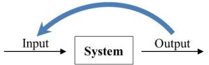
Earlier we said that systems are responsive: what they produce is a function of what they receive. However, we did not pay much attention to the origin of those inputs. Although a second system is often the source of factors entering one system, it is not impossible for a system to provide factors to itself—something produced by a system can actually re-enter and affect that same system. This phenomenon in which a system responds to its own outputs is referred to as feedback (see Figure 2.8), and the connection between what goes out and what goes in is sometimes referred to as a feedback loop. Feedback can bring about one of two very different outcomes, both of which play critical roles in the behavior of many systems (environmental and otherwise).
Negative feedback
With respect to a particular factor or factors, this first type of response will keep a system from changing much relative to its initial conditions (i.e., its starting point). How does negative feedback work? In short, output released now becomes new input later and counteracts actions of a system brought about by previous inputs. We can think of negative feedback as a mechanism by which current system response can cancel out previous system responses, or, put another way, regulate or reverse any movement away from its initial conditions. This somewhat murky concept becomes clearer if we consider a familiar system that is regulated through negative feedback. Climate control of interior spaces provides an excellent example of the principles of negative feedback. First, consider the goal of such a system: we want it to keep the temperature of the air in a room at some level we deem to be appropriate. Second, imagine how we might go about achieving our goal. Somehow, whenever there is a change away from the temperature we desire, often referred to as the set point, we would like the system to respond such that the change is reversed. If it gets too cold, we want the room to get warmer, and if it gets too warm, we want it to get cooler. Think about how you would design a classroom to maximize comfort (presumably, to minimize distraction from learning, not to induce sleep). Among other properties, we could decide that the ideal temperature is 20 °C (68 °F). So we include a climate control system that has the ability to both cool (i.e., air conditioning) and warm (i.e., heat) the space as needed. In this case let us assume our thermostat detects that the air it draws inside itself is 19 °C. That input, air temperature, triggers a response, and the heater is activated. Eventually, the temperature of the air in the room will rise to 20 and then 21 °C. At that moment, the changed input (i.e., air that is warmer than the set point) brings about a new response: the heater is turned off and the air conditioner is turned on. That system response will continue until the air is cooled below the set point and the heat will come back on once again. The result is a room that is maintained at a stable temperature indefinitely—there is little or no change. Figure 2.9 shows how our system model helps to visualize climate control.
Human body temperature is also stabilized through negative feedback. People will sweat if they get too hot (say, while running a race) and will shiver if they get too cold (say, while swimming in a chilly lake or after prolonged sweating). Whenever the body’s internal thermostat detects a deviation from optimal conditions, 37 °C (98.6 °F), its response is to reverse the change. Negative feedback controls a large number of processes relevant to environmental science, as we will see in upcoming chapters.
Positive feedback
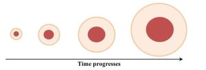
In this second case, the system response to its own outputs leads to changes with respect to a particular factor. Importantly, as feedback continues, the system moves farther and farther from initial conditions at an ever-increasing rate. Unlike negative feedback, current output becomes new input later that accentuates actions brought about by previous inputs. Again, examples will help us better understand this complex idea. We will start outside of the sciences with an adage: “it takes money to make money.” It turns out this expression is a nice way to summarize how positive feedback can increase the amount of money in a bank account. Say you deposit $1000 into a bank that pays 5% annual interest on your balance. Importantly, the interest is compounded, meaning that the amount earned in interest is added to the principle, and that combined amount is then used to calculate how much future interest is paid. Keeping things simple, a 5% return on your initial investment would yield $50 after a year. In the second year, though, the bank would pay interest on $1050 (the principle plus the interest earned in the first year), which is $52.20, so after two years you would have $1102.20. After three years, the account value would be $1157.62, and so forth. The more money you have, the more money you will make, and the faster your savings will grow. A second example closer to the subject of this book is how positive feedback can cause forest fires to spread. Visualize what could happen to a slightly damp forest if a seemingly inconsequential ignition source (maybe a lit cigarette) is released into it: a rather small area will start to burn. After a short time, combustible material in the vicinity will get dried out due to the heat from the fire, and it too will ignite. Now a larger area than we saw initially is burning. That larger fire will heat and dry additional material, but at this stage the amount dried and prepped for a fire is larger because the size of the fire has increased. As the fire grows, it will dry material at an ever-increasing rate and therefore grow at a similarly accelerated rate (Figure 2.10). Put into casual language, the bigger it gets the bigger it will get.
Population growth is another important phenomenon fueled by positive feedback. We will see this in more detail in Chapter 8, but for now consider how a small population can rapidly increase in size as it grows. In principle, the actions of just a few parents can ultimately lead to a very large number of descendants. For the sake of argument, we imagine a population consisting of three breeding pairs (six total individuals) that each produces four offspring. After one generation, the number of individuals will be 12. Keeping things simple, those offspring will eventually mature and pair up to produce their own offspring. If they behave like their ancestors, each of the six couples will give rise to four offspring, and the resulting population will consist of 24 new individuals (plus some survivors from previous generations). Under idealized conditions of infinite resource availability (not realistic, of course), the same pattern will repeat, and positive feedback will produce a constant rate of increase known as exponential growth. Put another way, the number of individuals in every generation can be multiplied by the same number to predict the size of the population in the future. A population that grows at 1% per year will add more and more individuals as the population gets larger and larger. Growth is a constant 1% of an ever-increasing number (e.g., 1% of 1000 the first year, 1% of 1010 the second year, and so on). See Figure 2.11 for a graphical representation.
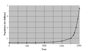
The same forces that drive compound interest (above) are active here: as the number of individuals capable of producing offspring grows, the number of individuals present increases at a faster and faster rate. As with negative feedback, we will see how positive feedback plays a role in many important environmental issues.
Three final points about feedback
Rate of change matters. Although it is tempting to view it as a phenomenon that always increases the size of a factor, note that positive feedback leads to an ever-increasing rate of change away from initial conditions. The observed change could yield either more or less output in the future. Consider the spread of a deadly disease, for instance. As more and more people are infected, the size of the population will decrease at an exponential rate. The same can be true of a melting glacier—as it gets smaller, the rate of shrinkage will increase because the low-temperature glacier keeps ice in its vicinity cool. Less ice leads to warmer temperatures near the glacier and even less ice in the future (Chapter 14). So, positive and negative feedback differ in that the former leads to instability and change whereas the latter brings stability.
Output must affect the system. It is critical to understand that the relationship between outputs and future inputs is a causative one. That is, a system moves back to (negative) or away from (positive) initial conditions as a direct result of output it just produced. To revisit two of our examples, a human body will cool itself because it was heated, and a forest fire gets bigger because of the drying action of an earlier fire. As we saw near the beginning of this chapter, correlation does not guarantee that two phenomena are mechanistically linked.
This is not about bad and good. The words “negative” and “positive” should not be read as value judgments. Negative feedback is so named because the output cancels out or negates the action of a system. The result could be either beneficial or harmful. Positive feedback leads to change, a result that could be a good or bad thing. In fact, stability is often good for living systems, and change can be deadly. We will see many examples of the effects of feedback on environmental systems in upcoming chapters, some of which we will interpret to be helpful and some we will likely decide are detrimental.
2.2.3. Relationship between rate in and rate out
The relative rates of input and output determine if the amount of a factor inside a system increases, decreases, or stays constant with time. This is an important consideration because, as we saw in Chapter 1, environmental scientists track the movement and storage of important materials on Earth. They often use the tools of systems analysis to predict the availability of resources vital to both humans and non-human organisms alike. We can identify three distinct possible relationships between the rate at which factors enter and those at which they exit from a system (Figure 2.12 and the text that follows).
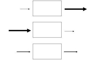
Rate of output could be higher than rate of input (top model in Figure 2.12)
In this case, we would observe depletion, a measurable decrease in the amount of material inside the system. Again, we will begin with a financial example. Investment accounts typically grow while the people holding them are employed and earning a salary. Workers contribute to them and their values increases. However, upon retirement, these accounts act as sources of income for those who created them. In all likelihood, the rate at which money is withdrawn will exceed the rate at which it is added. We will see depletion on a number of occasions during our study of Earth’s natural systems. Dwindling reservoirs of water, fuel, and fertile land are only three examples we will consider.
Rate of input could exceed rate of output (middle model in Figure 2.12)
Unlike the outcome of our first case, the factor under investigation accumulates, meaning there is an appreciable increase in the amount of the material inside the system with time. A familiar example from outside of the sciences is a savings or investment account. In short, we wish to see an increase in the amount of money inside the system—your portfolio, in this case—with time. This goal can be met by simply adding money faster than you withdraw it. Of course, the compound interest and positive feedback we considered previously will only increase the rate of input over that of output. Environmental scientists would be interested in this model as well, particularly if accumulation leads to damage of a system. A small pond could receive pollution far faster than it is able to process and discharge it, for instance, so the toxic material will accumulate.
Rates of input and output could be equal (bottom model in Figure 2.12)
In this case, there is flow through a system, but the net amount of a material inside the system does not change with time. Whatever exits is exactly replaced by new inputs. The term steady state is often used to describe this case. Is there a relevant example from the financial world to illustrate this case? When might we be interested in maintaining the amount of money in an account with no net increases or decreases? Checking accounts generally are designed to discourage both accumulation and depletion in the long run. Since little or no interest is paid on these types of accounts, there is no incentive to keep more money in there than is necessary to cover expenses (say, all the withdrawals made in a month). Depletion is also undesirable, though, as the inconvenient and costly phenomenon known as overdraft is the result. If your balance drops below the amount needed, your bank probably will assess a fee to you as a penalty. The steady-state model is important to environmental scientists because it is linked to the concept of sustainability we encountered in Chapter 1. Depending upon how they are defined and how long they are observed, some systems can be appropriately classified as steady state. For example, water in one small region might seem to be accumulating while it is depleted in another, but there is no change in the total amount of water on Earth. Practices such as tree farming in which harvesting is exactly offset by replanting could be viewed as steady state for a relatively short period of time. As we will see later, though, systems in which we cultivate plants of any type are subject to a reduction in how much growth can be supported in the long run (Chapter 9). Changes can also occur in the short run because materials are removed from systems at rates that are either higher or lower than those responsible for replenishing them. A related concern is the concept of residence time, that is, how long a material will persist in a system (see Box 2.4). We will return to input-output analysis and how it informs our understanding of resource availability throughout this book.
Box 2.4. Residence time: how long will stuff stay in a system?
Environmental scientists often wonder just how long a factor of interest will be present inside a system at steady state. If the material is required by organisms, we want to know if it will be present for sufficient time to support growth and survival. Sometimes the material is toxic, however, and the longer it stays inside a system the more opportunities it will have to cause harm. If we know the size of the pool, that is how much material is in a system, and the rate at which the material in question passes through that system (at steady state, either the rate of input or output provides the answer), we can use the following formula to determine residence time:
Amount in reservoir ÷ rate of outflow (or inflow) = residence time
Let’s use a simple and familiar example to get a sense of how this works: the length of time it takes a typical undergraduate to earn a Bachelor’s degree, or the residence time of a college student on a campus. Imagine a hypothetical college with a total of 2000 undergraduates and a graduating class of 500 each year. Residence time is therefore
2000 students ÷ 500 students / year = 4 years.
An environmental scientist might ask a seemingly more urgent question such as, what is the residence time of a harmful pesticide in a pond? If the size of the pond is 100,000 gallons (378,541 liters) and the rate of input is 1000 gal (3785 L) per month, then residence time is
100,000 gal ÷ 1000 gal / month = 100 months.
How is this information useful? If we know residence time of a toxic substance we will have an idea of how long it will take to clean up the affected system. Pollutants with shorter residence times are likely of lesser concern than those that persist for long periods.
THE CHAPTER ESSENCE IN BRIEF [1]
The scientific method provides a framework to collect evidence and increase our understanding of the natural world. It is objective, collaborative, and holds itself to high standards. Additionally, the simple set of tools of systems analysis allows us to assess the movement and storage of materials as well as the relative stability of many different phenomena.
Think about it some more…[2]
Why is the scientific method useful? What’s the point of such a complex set of steps?
How can you distinguish between an objective observation and a subjective one?
How would you react if someone says “your opinion is wrong!”?
Is scientific uncertainty an indication that scientists do not know what they are talking about?
Is it possible to obtain highly precise measurements if you use a scale that is poorly calibrated?
How could pollution of a pond be a good example of an imbalance between inputs and outputs as well as positive feedback?
- As you will find throughout this book, here is very succinct summary of the major themes and conclusions of Chapter 2 distilled down to a few sentences and fit to be printed on a t-shirt or posted to social media. ↵
- These questions should not be viewed as an exhaustive review of this chapter; rather, they are intended to provide a starting point for you to contemplate and synthesize some important ideas you have learned so far. ↵
An approach that is characterized by values and biases; contrast with objective. See Chapter 1 for more.
A systematic strategy used by scientists to answer questions about the natural world. It is designed to facilitate objectivity and repeatability. The specific steps used by scientists different somewhat among disciplines, but they generally include some variation on: observation, hypothesis, experimentation, conclusion, repeat / refine hypothesis, share information with the scientific community. Chapter 2 contains a detailed description.
A strategy used by scientists in their study of the natural world. It involves the observation of specific, representative phenomena to develop general conclusions or rules that govern the universe. See Chapter 2 for more.
A strategy used by scientists in which specific cases are compared to previously developed and accepted principles. It is often used to categorize organisms or objects into preexisting groups. See Chapter 2 for more.
Controls or control subjects help establish causation. These are subjects that are untreated in an experiment; in other words, they provide the baseline against which test subjects are compared. Controls are essential to experimental science. If controls and test subjects respond the same way, the factor tested likely is not responsible for the reactions noted. See Chapter 2 for more.
In geology, describes how the lithosphere of Earth is broken into several units called plates. These plates slowly move horizontally with respect to each other. Plate movements are responsible for continental drift, earthquakes, volcanoes, and other important phenomena. See Chapter 3 for details.
Holds that populations change with time in response to a number of factors, including mutations, natural selection, and random chance. Biological evolution is the main scientific explanation for the development of life on Earth. See Chapter 6 for many more details.
Describe how energy is used and converted among forms (e.g., potential, kinetic, and heat). See Chapter 4 for details.
A property of any scientific measurement, it represents the size of the error term for a measurement. Can be thought of as the range of possible answers to a question (often, from lowest to highest). May be expressed as a number, e.g., 5.0 +/- 0.5 which indicates an average value (or otherwise representative number) of 5 with a possible range of 4.5 to 5.5. It arises from random and systematic errors. See Chapter 2 for more.
The correctness of a measurement in relation to a universally accepted standard. Contrast with precision and sensitivity. See Chapter 2 for details.
A procedure to assess the accuracy of a scientific instrument. Accomplished by measuring a standard of known properties. For example, a balance could be calibrated through the use of a calibration weight, a carefully constructed object of known mass. A calibration weight with a mass = 1.00000 g could be used to assess the accuracy of a laboratory balance; if the mass of the object is determined to be 0.99880, we know the balance needs to be calibrated. Put informally, we need to remind the balance what 1.00000 g actually looks like! See also accuracy and Box 2.2.
How well multiple readings, or replicates, of the same phenomena agree with each other. Contrast with accuracy and sensitivity. See Chapter 2 for details.
A shorthand word often used by scientists to refer to multiple measurements of the same phenomena: each reading is a replicate. Put another way, we replicate or repeat a measurement multiple times. See also precision. See Chapter 2 for more.
Refers to the many different kinds of microscopic organisms that are single celled and prokaryotic (i.e., do not possess distinct cellular organelles). Collectively, bacteria are extremely diverse, are the oldest organisms on Earth, and are critical to many environmental cycles and processes. See Chapter 3 for more.
