14 Air Pollution and Climate Change
Jason Kelsey
Many of the natural processes and human activities we have studied in previous chapters release pollutants into Earth’s atmosphere. Here we examine several important consequences of these emissions. Note that some of the most politically charged topics in this textbook are part of Chapter 14, so we should be particularly careful to maintain our objectivity, seek evidence-based explanations, and stay firmly grounded in science. Various scientific arguments will be considered, but unscientific arguments will not receive equal attention (review Chapter 2 for more about science as a way of knowing).
Key concepts
After reading Chapter 14, you should understand the following:
- The many sources and types of atmospheric pollutants
- Why humans intentionally pollute the atmosphere
- The three scales of air pollution
- The causes and consequences of smog
- How acid precipitation forms, why it is of concern, and how it can be mitigated
- The evidence supporting the claim that human activity is changing global climate, why climate change is problematic, and how it could be combatted
- The causes and consequences of ozone depletion, a phenomenon largely separate from climate change
- How global cooperation among Earth’s nations has allowed the ozone layer to partially recover
- The connections among fossil fuel combustion (Chapter 10) and outdoor air pollution
- How indoor environments are subject to air pollution
14.1. AN INTRODUCTION TO ATMOSPHERIC POLLUTION
14.1.1. The atmosphere is dynamic
We begin with a brief reminder of the characteristics of the atmosphere. In simplest terms, it can be visualized as several layers of gases that envelop the solid planet. It is intimately linked to the hydrosphere, biosphere, and lithosphere, as the four spheres affect and are affected by each other. Gases here move and mix, and their composition has changed throughout history due to the activities of terrestrial and aquatic organisms. You are strongly encouraged to review the first several pages of Chapter 4, including Figure 4.1, for more information about the structure, chemistry, and processes active in the atmosphere.
14.1.2. Many substances can pollute the air
Air pollutants can be defined as substances that enter the atmosphere and lead to adverse consequences. Since their origins and properties are so varied, environmental scientists have established categories of pollutants based on answers to several simple questions.
Chemical, physical, or biological?
This categorization scheme groups substances based on their fundamental nature and the resultant types of risk they pose when in the atmosphere.
Chemical. Chiefly due to their chemical properties, these pollutants can directly or indirectly affect organisms and ecosystems.
Direct effects
Many substances are emitted from sources in forms that are immediately toxic. For example, mercury and sulfur dioxide from coal combustion can cause brain damage and lung irritation, respectively.
Indirect effects
Some substances are transformed to new chemical pollutants via reactions they undergo in the atmosphere. Sulfur dioxide, seen above as acting directly, also can react to form sulfuric acid and cause acid rain (described shortly). Alternatively, a substance in the air could be of concern not because it reacts to form a new chemical entity, but because its presence leads to important modifications to environmental conditions. Carbon dioxide, for example, is generally innocuous—we humans spend our lives in the constant presence of this gas without experiencing any adverse health effects because of it. However, if an unusually large amount is suddenly introduced into a system, it temporarily displaces O2 such that all aerobic life forms in the affected region die from asphyxiation. A small number of volcanic events (Chapter 7) have killed herds of animals, as well as their human shepherds, through this unusual and deadly mechanism. On a much larger scale, CO2 also influences the average temperature of the Earth. As we will learn in some detail near the end of this chapter, increases in the amount of carbon dioxide in the atmosphere can be linked to changes in climate across the planet. Again, the gas does not act like a poison per se, but it still has the potential to appreciably affect living and non-living systems.
Physical. These substances also act directly and indirectly on the biosphere. For example, certain particles (e.g., fibers, fine dust, soot) can directly damage lung tissues, whereas large clouds of dust (e.g., from a volcanic eruption) can partially block incoming sunlight, drive changes to climate and, thus, indirectly affect organisms.
Biological. Cells of microorganisms (Chapter 3) may be sent into the air by natural forces such as sneezing, coughing, and the crashing of waves onto rocks, or through anthropogenic activity like manure spreading for agriculture (Chapter 9). Additionally, fungi and many plants launch spores and other structures into the atmosphere as part of their reproduction. If inhaled, these biological entities can cause harm to animals, including diseases and allergic reactions.
Natural or anthropogenic?
Air pollutants can originate from natural processes like decomposition and volcanic eruptions as well as from agriculture (Chapter 9), fuel combustion (Chapter 10), waste management (Chapter 13), and other human activities. This distinction is important for two reasons. First, many assume that harmful emissions come exclusively from people, but air pollution is a phenomenon that predates human civilization. Second, governments can only enact laws and policies to regulate anthropogenic sources of emissions—it likely goes without saying that we cannot prosecute or fine volcanoes whenever they release excessive amounts of hazardous gases. The focus of this chapter will be human sources of pollutants because those are the ones over which we can exert some control.
Mobile or stationary?
Here we distinguish between sources that move around, such as cars and trucks, and those that stay in one place, such as coal-burning power plants and volcanos. Why do we care about this difference? It comes down to ease of monitoring and controlling. Since, by design and intention, vehicles travel from place to place, it can be difficult to track the pollutants they are releasing. Standards vary among countries and U.S. states, but it is safe to say that a car could produce an enormous amount of pollution, far more than is legal, before the problem is discovered. On the other hand, emissions from a fixed smokestack are relatively easy to test, meaning violations of regulations can be readily detected.
Primary or secondary?
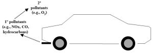
This categorization scheme reflects whether a substance has been chemically transformed after release from its source. A primary pollutant is one that has not been altered from its original form, whereas a secondary pollutant is the product of reactions involving primary pollutants. Consider, for example, the exhaust from a car: it consists of several primary pollutants, including carbon dioxide, carbon monoxide, various hydrocarbons, and compounds containing nitrogen or sulfur. It turns out that each of these chemical substances is potentially problematic in its own right. However, on hot, sunny days, a secondary pollutant called ozone gas can be produced in reactions involving some of the components in the tailpipe emissions (Figure 14.1; we will also return to this point shortly).
As we saw above, the utility of these designations can be understood in the context of regulations. Laws about allowable amounts and types of primary pollutants from different sources are influenced by many factors, including the likelihood that secondary pollutants will be produced. These pollutant types play roles in upcoming sections of this chapter.
Indoor or outdoor?
Pollution is not a phenomenon affecting only open-air environments, as some of the most serious air quality problems are found in closed, interior spaces like factories, laboratories, and offices. As you likely expect, rules about the composition of indoor and outdoor air vary considerably. We will see specific examples of both types of air pollution later.
14.1.3. Pollutants are shared
Air moves fast
Everything on Earth is connected, as we have seen in many places throughout this book (review the principle of environmental unity, Chapter 1). However, since air is the fastest moving medium on this planet, atmospheric gases are more directly and obviously shared than are any other materials on the planet. In other words, substances emitted into the air can quickly spread from their sources and affect ecosystems and people thousands of kilometers away.
Air readily crosses political boundaries
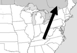
A somewhat simple and obvious fact is critical to our discussion of air pollution: lines drawn on maps do not stop air and the pollutants carried in it from moving among cities, states, and countries. Consequently, even if a local government passes the most rigorous air quality regulations, it will still be subject to the pollutants emitted by its less careful neighbors (Figure 14.2).
14.1.4. Erroneous assumptions about the atmosphere influence our actions
Humans have used the atmosphere as a receptacle for waste materials for centuries, despite knowing that polluted air is detrimental to human health. Why would we deliberately degrade such an important resource? The answer is driven by several assumptions, notions that are at least partially false.
Assumption 1: the atmosphere is so vast we cannot affect its composition
Recalling the adage “dilution is the solution to pollution” (Chapter 11), many people assume that human activity is incapable of appreciably changing the chemistry of Earth’s enormous atmosphere. The fact is, though, the atmosphere is not infinitely able to dilute air pollutants. We will see that the concentrations of numerous substances released from anthropogenic activities have measurably increased since the latter part of the Nineteenth Century.
Assumption 2: fast-moving air will make pollutants go away
Air currents have the capacity to rapidly carry pollutants away from their sources. The assumption, then, is that the risk of poisonous substances disappears in the wind. Two important problems challenge the validity of this expectation, however. First, again recalling the discussion of water pollution in Chapter 11, “out of sight, out of mind” fails to account for the reality of a shared atmosphere. Second, as we will see when we explore the problem of urban smog, later, pollutants do not always move away as we hope.
Assumption 3: chemical reactions reduce the toxicity of air pollutants
It is certainly true that chemical pollutants can be transformed via naturally occurring chemical reactions in the atmosphere, but those reactions do not necessarily eliminate toxic substances. Sometimes, they make matters worse. Urban smog and acid precipitation are two examples of problems associated with products of reactions, that is, secondary pollutants.
Assumption 4: the risk of air pollution is greatly exaggerated
Finally, many people are comfortable emitting potentially toxic substances into the atmosphere because they simply do not accept the conclusions of scientists. Resistance to reducing or eliminating certain pollutants is often driven by denial of data and evidence, an issue that is particularly problematic in the public discourse about global climate change (which we will explore later). Moreover, the effects of air pollution are sometimes seen as remote, trivial, or just a vague concern for subsequent human generations. Convenience and expedience in the here and now (along with, frankly, ignorance) can outweigh concerns about future adverse consequences.
14.1.5. Effects of air pollution vary with scale
The effects of outdoor air pollution are grouped into one of three categories: local (i.e., felt in the immediate vicinity of a source), regional (i.e., within several hundred kilometers of a source), and global (i.e., the entire planet). Specific examples of each level will be presented in the next section. Before we proceed with that discussion, though, you should realize that a single source of pollution can bring on effects at all three scales and that the nature of the observed consequences will likely be different at those different scales. We do not simply see the same phenomena affecting increasingly large areas, instead, we can observe one type of problem at the local scale, another at the local scale, and a third at the global scale. For example, emissions from one coal-fired powerplant (Chapter 10) can cause smog at the local level, acid precipitation regionally, and contribute to global warming, ocean acidification, and planet-wide climate change.
14.2. SOURCES AND CONSEQUENCES OF OUTDOOR AIR POLLUTION
The bulk of this chapter will address several local, regional, and global consequences that arise from the emission of pollutants into Earth’s atmosphere.
I: Local-scale effects
14.2.1. Smog
Local-scale effects are limited to areas close to air pollution sources. Of the phenomena that can be categorized here, we will consider only smog, an important problem seen in many urban areas.
What is smog?
The word “smog” was coined about a century ago as a contraction of “smoke” and “fog”. Since it is a moist, smoky, and cloudy mix of substances that impairs breathing and vision, this word is reasonably descriptive, if inexact. These days we use a more rigorous definition of smog, one that consists of two parts.
It accumulates near pollution sources. Smog defies the expectation described above that air currents will carry pollutants away from their sources. Several forces can trap smog in an area, as we will see below.
It consists of primary and secondary pollutants. Emissions from motor vehicles, factories, and power plants, including sulfur and nitrogen gases, hydrocarbons, and particulates, make up the bulk of the primary pollutants in smog. Ozone gas, O3, is a secondary pollutant derived from nitrogen dioxide (NO2) and hydrocarbons in intense sunlight. Again, we hope chemical reactions will reduce or eliminate the hazards of air-borne toxic substances, but in this case, they generate a new danger.
Factors promoting smog formation
High source density. Smog is most likely to develop where air pollution sources are concentrated. Cities, with their dense populations, large number of fossil-fuel burning vehicles, and manufacturing and power-generating facilities, are susceptible to smog.
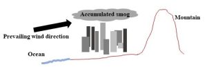
Topographical barriers. Air movement can be impeded by valley walls, mountains, and even steady wind blowing in one direction (Figure 14.3). As a result, some locations are simply more vulnerable to smog accumulation than are others.
Atmospheric inversions. These can restrict the movement of air pollutants away from sources and contribute to the problems of smog.
Vertical movement of air is inhibited
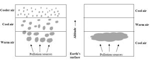
Air temperature usually decreases with altitude from the ground to the top of the troposphere (about 12 km high; review Figure 4.1). So, the warmest air—that at Earth’s surface—carries air pollutants up as it expands and rises. Cooler air at higher altitudes then drops (since it is denser than the warm air). Sometimes, though, a layer of cool air can sink below warm air and remain at ground level. This abnormal condition, known as an atmospheric or thermal inversion, traps air pollutants near their sources (Figure 14.4). Smog continues to accumulate as long as an inversion remains in place and vertical mixing of air is prevented.
Natural phenomena exacerbate anthropogenic activity
Thermal inversions occur naturally. For example, cooling under a clear night sky could cause cold air to sink and displace warm air sitting on the ground. A city located in an affected basin would then be subject to smog because the pollutants generated by its dense human population cannot disperse.
Appropriate climatic conditions. Since smog occurs under a specific set of atmospheric and climatic conditions, the severity and nature of it vary considerably with location, weather, and season.
Photochemical smog (Los Angeles smog)
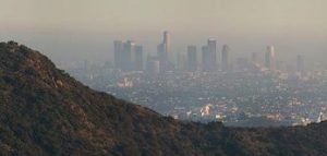
This type of smog is favored in hot, sunny, and dry locations. It tends to form when primary pollutants from cars and trucks are released into air and react in intense sunlight to form secondary pollutants. If winds are minimal or air movement is otherwise impeded, this toxic mixture of particulates, hydrocarbons, nitrogen oxides, and ozone can be trapped over a city until a new weather pattern brings relief (individual episodes of intense smog have been known to persist for several days). Many cities around the world are susceptible to photochemical smog formation. For example, Los Angeles, California (U.S.A.) often experiences this local air pollution problem because it possesses all the necessary ingredients: high source density from automobiles, manufacturing, and power generation, topographical boundaries, and ideal climatic conditions (generally high temperatures, low moisture and cloud cover, and minimal wind) (Figure 14.5.a).
Mexico City (Mexico), Beijing (China), and Santiago (Chile) are just three of the many other places that regularly endure photochemical smog.
Sulfurous smog (London smog)
Named for a city susceptible to it, sulfurous differs from photochemical smog in two important ways.
It occurs in areas that are cold, overcast, and wet. In these cases, sunlight is partially blocked from reaching the surface by heavy cloud cover. Less sun penetration causes ground-level air temperature to decrease and that in the atmosphere, at and above the clouds, to increase. Eventually, water condenses in the cooling air, and fog forms at the surface. Any air pollutants present will be unable to move very far from their sources; instead, they will accumulate.
Coal emissions play a major role. Here, smog often consists of primary pollutants from coal combustion, namely soot, hydrocarbons, and sulfur oxides. Because the conditions are not conducive to its formation, ozone is a minor concern. However, another secondary pollutant, sulfuric acid, may be produced. Combining the previous two points, we can imagine how sulfurous smog can become a serious problem. In response to falling air temperatures, people burn more coal to generate heat. As emissions accumulate, air quality worsens until weather conditions change and the inversion is disrupted. London (England) is well known for its susceptibility to this type of smog, even as coal usage there has declined during the past several decades (Figure 14.5.b).

Adverse effects of smog
Environmental health. Animals and plants can be inhibited or killed by exposure to smog. For example, lichen disappear from the sides of buildings in cities with serious smog problems. The loss of lichen in urban areas is often used as an indicator of poor air quality.
Human health. Several pollutants in smog are toxic to humans and can cause conditions ranging from mild irritation to death. Sulfur dioxide and ozone, for example, damage eyes and lungs and are deadly at high concentrations. Those with pre-existing respiratory conditions such as asthma are particularly vulnerable. During severe smog events, people generally avoid outside air as much as is possible.
What can be done about smog?
We will return to a broader discussion of air pollution prevention near the end of this chapter, but for now we will provide a simplistic, if reasonable, answer to the question: reduce emissions of primary pollutants such as those released during fossil fuel combustion.
II: Regional-scale effects
14.2.2. Acid precipitation
These effects are felt some distance away from the pollution sources that cause them. Acid precipitation, an important and familiar example of a regional-scale phenomenon, often occurs many hundreds of kilometers (or more) downwind of the sites from which the relevant emissions are released.
An introduction
Put simply, the name of this phenomenon says it all: air pollution causes rain, snow, ice, and fog to be more acidic (have a lower pH) than they would be otherwise. Dry materials can also be affected. Consult Box 14.1 for a short primer about the meaning and measurement of acidity.
Box 14.1. pH: how we measure and express acidity.
We already encountered the concept of acidity back in Chapter 9, but here we return to it in the context of air pollution.
The pH scale is used to express the acidity of water-based, or aqueous, liquids. In short, the amount of positively charged hydrogen ions (H+) present is measured and that number is converted to pH units. Acids have the highest concentrations of H+, and, because of the nature of the mathematical transformation used, the lowest pH values. Bases, on the other hand, contain more of a different ion, OH- (and lower amounts of H+), and have higher pH values. Although it can go beyond these limits, the scale usually is assumed to start at 0 (most acidic) and run to 14 (most basic). A liquid that is neither acidic nor basic, neutral, has a pH of 7 (Figure 14.6 shows the pH scale and includes values for some common substances).
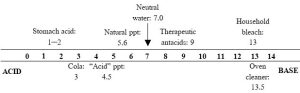
You should be aware of three critical facts related to the pH scale. First, the concentration of H+ ions does not change in a linear fashion, despite what Figure 14.6 suggests. Instead, each number represents a ten-fold change in acidity! Thus, the concentration of H+ in a liquid with a pH of 6 is ten times higher than that in a liquid having a pH of 7, pH 5 is ten times more acidic than pH 6, and so on. Furthermore, since each step in the scale multiples the difference in acidity by ten times, pH 3 indicates a concentration of H+ ions that is 1000 times higher, or is a thousand-fold more acidic than, pH 6 (10X for each step from 6 to 5 to 4 to 3). A change from, say, pH 5.5 to pH 4.5, is therefore more significant than it might appear. Second, when an acidic substance contacts a basic one, a reaction between the two will yield a more neutral (closer to pH 7) product. Anyone who has ever tried to relieve symptoms of heartburn by chewing antacids has experienced such a reaction firsthand: stomach acid escaping into the esophagus can be neutralized, albeit temporarily, by swallowing calcium carbonate or another basic substance. Finally, both acids and bases are corrosive—the further a substance is from pH 7, the more hazardous it is.
Origins and development of acid precipitation
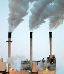
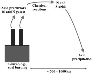
Acid precursors are emitted. The formation of acid precipitation begins with the release of certain primary pollutants into the atmosphere. Sulfur-oxygen compounds like SO2 emitted from coal-fired power plants (Figure 14.7), and nitrogen-oxygen compounds (i.e., “NOx” ) from gasoline, diesel, and coal burning (Chapter 10), are two important acid precursors. Natural sources of precursors, including volcanoes, also contribute.
Chemical reactions produce acids from acid precursors. Once in the air, the S and N gases can be converted in reactions with atmospheric water to nitric acid or sulfuric acid, respectively (Reactions 14.1, 14.2a and 14.2b).
(Reaction 14.1) 2NO2 + H2O → HNO2 + HNO3 (nitric acid)
(Reaction 14.2.a) SO2 + H2O → H2SO3 then,
(Reaction 14.2.b) 2H2SO3 + O2 → 2H2SO4 (sulfuric acid)
Both nitric and sulfuric acid dissolve into precipitation and lower its pH. You should realize that, due to chemical conditions in the atmosphere, unpolluted natural rainwater has a pH of about 5.6; in other words, it is already somewhat acidic. To be classified as true acid precipitation, pH has to fall to 4.0 or lower (take another look at Figure 14.6, above). Figure 14.8 provides a graphical overview of the steps that lead to this regional air pollution problem.
Potential adverse effects of acid precipitation
Several consequences can be caused by acid precipitation. As we will see in the next section, though, the severity of the described effects varies from place to place.
Environmental health. Because it can dramatically alter the chemistry of soil and water, acidic precipitation may influence the structure and function of ecosystems (Chapter 5). If the changes are moderate, acid-tolerant species can gain an advantage over those that have adapted to higher (and what we could reasonably consider to be normal) pH. More severe acidification may create environmental conditions that few organisms survive.
Terrestrial
Forests, grasslands, farms, and other land-based systems rely on soil for nutrients, water, and physical support (Chapters 5 and 9). Changes to soil pH can reduce the success of plants and pose a challenge to all organisms present in an affected area. Importantly, the acids do not tend to harm plants directly, rather they introduce stress by disrupting the physical structure of soil, initiating reactions that increase the biological availability of toxic metals (e.g., aluminum), and decreasing the amount of essential nutrients present. Forests populated by trees that were otherwise well adapted to their environments and able to withstand stressors such as herbivory (i.e., consumption by plant-eating animals) and diseases have been severely damaged following substantial increases in the acidity of precipitation.
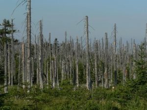
Portions of southern Germany and southeastern Canada, along with northeastern states such as New York and Vermont (U.S.A.), are among the places in which acid-related forest damage is prevalent (Figure 14.9). Production of crops from agricultural fields (Chapter 9) can also be reduced in acidified soils.
Aquatic
Acid precipitation can lower the pH of lakes and rivers to levels that are quite hostile to native organisms. Increased acidity can directly damage anything not adapted to such conditions, but indirect effects are at least as important. For example, the extra mucous some fish produce in response to stress can interfere with oxygen uptake through gills and even kill through asphyxiation. Acids can also lead to loss of nutrients (through chemical reactions like those seen in soils, above), inhibiting primary producers. Aquatic communities in the Adirondack Mountains of New York (U.S.A) provide just one example of the potential damage this regional phenomenon can cause. Historically, precursors released from coal power plants in places such as Ohio and Pennsylvania moved northeast and acidified precipitation in upstate New York. The pH of lakes fell precipitously, leaving many visibly barren. Certain rivers in Oslo (Norway) have undergone similar chemical changes, leading to declines in the numbers of important species such as salmon.
Susceptibility to acid precipitation varies
Acid precipitation does not lead to the same consequences everywhere. Due to several environmental factors, including a property known as buffering capacity, separate locations receiving the same acidified rainfall may respond quite differently. Put simply, buffering capacity is the amount of acid or base a material can absorb before its pH changes. So, something that can withstand the addition of large amounts of acid without itself become appreciably more acidic is said to have high buffering capacity. Low buffering capacity would be the term used to describe something that is very sensitive to (i.e., easily changed by) a small amount of acid. Limestone and related rocks are largely comprised of the compound calcium carbonate, an important natural buffer. If soil in a forest, field, or other terrestrial system was derived from such materials (see Chapter 9 for information about the contributions rocks make to soil formation), its pH will remain relatively constant even as it receives large amounts of acidic precipitation. A body of water can also be stabilized if its sediments contain calcium carbonate or similar compounds. Since granite, sandstone, and most other common rocks have very low buffering capacity, the pH of systems containing them, or products of their weathering, are easily lowered by incoming acids. Interestingly, the pH of water within the same stream can differ substantially from place to place—within just a few km—as the types of rock underlying it change. The Bushkill Creek in Eastern Pennsylvania (U.S.A.) provides a good example of this phenomenon, with its pH rising from approximately 6.5 to 7.5 as it flows a mere 20 km. Finally, keep in mind that, although resistance to pH changes can provide a benefit to humans, high buffering capacity may increase the numbers of sinkholes in an area (see Box 14.2 for more).
Box 14.2. Getting swallowed by the Earth: a price of high buffering capacity?
There can be a downside to the presence of good natural buffers like limestone in—and more importantly, under—an area: the neutralization reactions of the acids in infiltrating water with the bases in the solid rocks providing support for the surface can create big problems. Eventually, if enough of the underlying limestone is dissolved, the ground can collapse into depressions called sinkholes (Figure 14.10a. and 14.10.b).


Sinkholes range in size from less than a meter across and a few centimeters deep to hundreds of meters in all dimensions. Sometimes they appear suddenly, imperiling unfortunate people in vehicles, buildings, or just standing at the wrong place at the wrong time. In other cases, they open gradually, allowing enough time for evacuations. You should be aware that many natural and anthropogenic activities (including unsustainable usage of groundwater—see Chapter 11) can bring about sinkholes, with acid-base reactions just one common mechanism. It may be possible to fix these holes using one of several approaches. The enormous levels of destruction and human suffering that can be caused by sinkholes should remind us yet again of the value of objective study and science: if decisions about land use, including where and how to build structures, roads, and bridges, are made without consideration of available knowledge and data, the consequences can be expensive and even deadly.
Responding to the adverse effects of acid precipitation
Humans can mitigate some of the consequences of acid precipitation in both natural and managed systems by taking advantage of the acid-base neutralization reactions described in Box 14.1, above. For example, a white, powdery substance commonly known as lime is often applied to acidified agricultural fields. The calcium hydroxide in this material reacts with acids, pushing soil pH up toward a more neutral value. Although it adds yet another task (and expense) to the life of a farmer, regular liming between growing seasons helps maintain crop yields that would otherwise be limited by acid-induced loses in soil fertility (Figure 14.11).

Reducing acid precipitation
As noted at the end of the section on smog, we will take up the larger topic of reducing air pollution, including emissions of acid precursors, near the end of the chapter.
III: Global-scale effects
Now we consider two consequences of air pollution that affect the entire Earth, in areas both close to and remote from emissions sources: climate change and ozone depletion.
14.2.3. Global climate change
The first item on our list is familiar to most people living in today’s world because it is discussed so widely. Furthermore, it is a controversial and divisive issue, eliciting intense, often values-based responses, from many people—including those with expertise in areas other than science. The reasons for the high levels of passion surrounding global climate change are numerous and include the fact that the problem is complex and difficult to understand, the potential consequences of it are enormous and dangerous, and the solutions we must embrace to reverse or minimize it range from inconvenient to very unpleasant. Here we will largely steer clear of politics and opinions about what we would like to be true about Earth’s natural systems and our relationships to them and examine the science of climate change.
We begin with the name: global warming or climate change?
Right off the bat, the name used to describe this phenomenon is complicated and, unfortunately, a source of some confusion and even suspicion. When it first became a well-known issue over three decades ago, this problem was generally called “warming” because it referred to an increase in the average temperature of the entire Earth. In more recent years, scientists have called it “climate change”, as that term more accurately reflects the relevance and consequences of global warming. In other words: we are still studying, and concerned about, changes in the planet’s temperature. However, it is critically important to realize that global warming does not cause the temperature in every location on Earth to go up. Instead, due to an overall higher temperature, individual climates across the globe shift and change. Although most areas would indeed become hotter, others would actually get colder. Precipitation patterns would also change, increasing or decreasing water availability in different ways in different places and ecosystems. In short, the problem is far more nuanced than is reflected in the original name. Some people who do not accept that climate change is a real concern (we will examine their arguments near the end of this section) point to this new name as a sign that the science of climate change is unreliable and invalid rather than an attempt to better describe the problem.
Questions of interest to scientists
The essence of this global-scale air pollution can be captured in four essential questions.
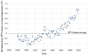
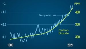
#1: Is Earth getting warmer? The very concise, and evidence-based, answer to this question is: yes. Widely accepted data indicate that the average temperature of this planet has gone up by about 1.1ºC (around 2º F) since the pre-industrial age (defined as 1880 – 1900)[1], but the rate of change has been neither uniform nor constant. Notably, most of the observed increase occurred during the past 35 years, with the warmest years on record (in descending order) being 2023, 2016, 2020, 2019, 2015, 2017, 2018, 2014, 2010, 2013 and 2005 (tied)[2],[3]; interestingly, the hottest single days on record occurred during July of 2023)[4]. Taking a somewhat longer view, most of the years 1900–1977 were cooler than the average for the 20th Century; since then, every year has been warmer than that same average (Figure 14.12).
Will this warming trend continue? We will see more about making predictions below, but for now, careful analysis of past, current, and expected future patterns points to an average global increase of 1.1 – 5.4 ºC (2 – 9.7 ºF) by the year 2100[5].
#2: If the answer to question #1 is “yes”, what is the cause? Although a small number of people argue otherwise, the temperature of the Earth clearly has gone up and appears likely to continue along that trajectory into the future. The data are reliable and difficult to dispute. With that first of our four questions relatively easily handled, then, we move on to our second, somewhat more difficult question. Given our observations that the average temperature on Earth has been going up for more than a century, it stands to reason that the rate at which energy enters this system currently outpaces the rate at which it exits. That is, either the amount of energy received by the planet has increased since 1880 or the amount of energy retained has increased during the same period. So, which has changed, inputs or outputs? To answer, we must examine three major factors that control Earth’s energy balance.
The sun’s energy output
You might be surprised to learn that the sun does not release a constant amount of energy. Instead, it cycles through periods of relatively high and low output. Decades of scientific study have revealed that visible changes to its surface are directly linked to the amount of energy it releases, with features known as sunspots coming and going as output waxes and wanes, respectively (Figure 14.13).
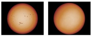
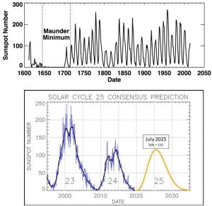
With the proper type of telescope, you can safely see and count the dark patches present at any moment. People have been doing this for centuries, and their data show something unmistakable: the cycles are regular, with the highest numbers of sunspots (referred to as maximum sunspot activity) appearing every 11 years. Figure 14.14.a shows the record of sunspot activity humans have kept since the early 1600s (note that modern scientists consider data from the first century of collection to be less reliable than those collected since), and Figure 14.14.b. shows the most recent data and a prediction for the next several years.
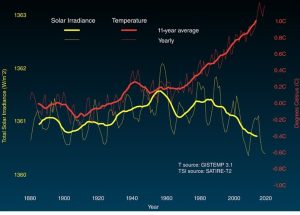
Fluctuations in the sun’s output are relevant to us because they might be responsible for the increased average temperature described in our first question, above. If recent changes in Earth’s temperature have been exclusively caused by changes in the sun, then the answer to the second question is “global warming is the product of natural forces over which humans have no control”, that is, we would be powerless to do anything about it except adapt. Indeed, some who deny the reality of human-caused climate change make such an argument. Although there is some on-going discussion of this point among scientists, most hold that the data simply do not support the sun-as-cause hypothesis for a few reasons. First, the Earth’s temperature has been going up since about 1880, and the rate of that increase has accelerated during the past few decades despite the ups and downs of energy received from the sun. Second, data from satellite sensors indicate no net change in the total solar energy received by Earth since 1978—even as Earth’s temperature has gone up (Figure 14.15).
Third, sun-driven warming should affect all layers of the atmosphere. However, evidence shows that only the inner atmosphere and the surface are warming (in fact, the stratosphere has been cooling recently), an outcome more consistent with an increase in the planet’s greenhouse effect (described below)[6]. Does a change in energy received affect Earth’s climate? It would be hard to imagine otherwise. However, forces that exert an even greater effect on temperature seem to be overwhelming fluctuating solar activity. Put succinctly, something else must be responsible for rising temperatures.
Earth’s albedo
The amount of incoming solar energy reflected off the Earth, its albedo, is a second potential factor controlling temperature. As we saw in Chapter 4, the color of a surface affects how much energy it absorbs: broadly speaking, lighter colors reflect more than do darker ones. Ice and snow absorb less energy than soil, dark rocks, and asphalt (green forests are somewhere between those extremes). So, we would expect this planet’s average temperature to be influenced by natural and human activities that alter surface characteristics. Below is a short list of specific phenomena that can change how much incoming solar energy is reflected off the planet to space.
Volcanic activity. We learned in Chapter 7 that eruptions release molten and solid rock, ash, and several gases into the air. Ash—a mixture of very small and light particles that can be distributed across the globe by wind and then stays aloft for years—is particularly important in this current context because it can block a fraction of sunlight reaching Earth. Major volcanic eruptions have brought about measurable cooling in their aftermaths throughout history. The 1991 eruption of Mt. Pinatubo in the Philippines serves as one example of the effect of volcanoes on albedo. The massive amount of ash and other materials ejected into the air was spread throughout the entire stratosphere within a year of the explosion and lowered average temperatures by about 0.6 ºC for the next 15 months. Once the materials dispersed and settled, the cooling effect disappeared[7].
Cloud cover. Water vapor in the atmosphere can interact with dust particles to form clouds, and these clouds can reduce absorption—that is, increase albedo—because they block some sunlight entering the atmosphere. Changes in the amount of cloud cover have the potential to affect the amount of energy reaching the Earth and its average temperature. When we discuss variables affecting the way scientists are able to predict the future of global warming, we will return to the subject of clouds.
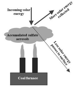
Anthropogenic air pollution. Certain emissions from human activity can affect albedo. For example, sulfur compounds and solid particles produced by coal combustion—sometimes referred to as sulfate aerosols—can enter the atmosphere and block some incoming radiation (Figure 14.16).
In a somewhat ironic and unintended outcome, efforts to clean up emissions from coal-fired power plants during the past few decades have led to a decrease in the cooling effects caused by particulate pollution. Few would argue that more toxic air on the local scale is therefore a good thing, but it is, nonetheless, a fact that cannot be ignored.
Land use changes. The spread of human civilization and advances in technology and standards of living (Chapter 8) have altered Earth’s surface during the past millennia. Large-scale changes such as the building of cities and conversions of hundreds of thousands of acres of forests to farms are two of the important ways we could change surface colors from light to dark and reduce albedo. The extent to which these changes have appreciably lowered albedo is unclear, though, and further study is underway to improve our knowledge.
To conclude this short discussion of albedo, we should acknowledge that the relative importance of changes in energy reflection to the larger story of contemporary global warming is not well understood. The phenomena described above clearly play roles, but whether they are strongly linked to the temperature changes observed since 1880 is by no means clear. Worth noting, however, is a NASA monitoring program that has so far revealed no compelling evidence for long-term change in global albedo[8], despite the well-documented, widespread clearing of land, expansion of agriculture, and urbanization that have occurred while average temperatures steadily went up. In any case, scientists continue to study the problem.
Heat retained by the atmosphere
Commonly known as the greenhouse effect, this final factor is extremely important to the living things on Earth as well as to the process of global warming. Here we look at this large, complex process, in small, relatively simple pieces.
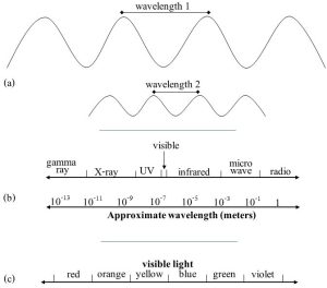
The atmosphere is transparent to some incoming solar energy. Earth receives several types of energy, known as electromagnetic radiation, from the sun. These different types are distinguished from each other by a property known as wavelength, the distance between the peaks or valleys of the travelling energy waves (Figure 14.17a). As represented by the electromagnetic spectrum (Figure 14.17b), wavelengths range from very short (about 0.000000000001 meters, m) to very long (about 10 m). Much of the energy emitted by the sun is in the range of 400 – 700 nanometers (nm, 0.000000001 m). These wavelengths can be seen by the human eye and are generally referred to as visible light. It is energy in this limited, visible range (Figure 14.17c), that easily passes through the gases in the atmosphere.
Incoming energy is converted to heat. Light energy striking the surface is converted into longer-wave infrared (IR), or heat energy, and then radiated up and outward toward space.
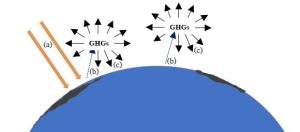
The atmosphere is relatively opaque to outgoing heat energy. Because longer-wavelength IR energy has different properties than light energy, it cannot easily pass though the atmosphere. Instead, the heat radiated from the surface is absorbed by certain tropospheric gases (called greenhouse gases, or GHGs) and then re-emitted in all directions—including back toward the Earth (Figure 14.18). We will return to the subject of GHGs, including their sources and concentrations in the atmosphere, shortly.
The greenhouse effect is natural and life giving. Although sometimes mistaken to be both a creation of and menace to humans, at the most basic level, the greenhouse effect is neither. Natural processes produced, shaped, and maintained it for many millions of years, long before any people appeared on Earth. We will see in upcoming discussions that the greenhouse effect can be altered by humans, but it was certainly not created through anthropogenic activity. Furthermore, the greenhouse effect is not a bad thing! In fact, because GHGs absorb and re-radiate heat, life as we know it can live here. Notably, the greenhouse effect increases the average temperature of the surface by about 33 ºC[9], meaning that water is present in all three phases (solid, liquid, and vapor). Earth would be far too cold without it for its current biosphere to exist.
The greenhouse effect was described nearly two centuries ago. Contrary to what is believed by many, the science of the greenhouse effect is hardly new. Scientists living in the 1800s studied the relationship between GHG concentrations and Earth’s temperature. In the 1850s, for example, a woman named Eunice Newton Foote was one of the first to discover that carbon dioxide plays a role in heating up a gas-filled atmosphere[10]. Others expanded on her findings, including a Swedish chemist named Svante Arrhenius, who, in 1896, conducted further work and even boldly suggested that human activity—notably, the burning of fossil fuels—would likely increase Earth’s temperature by adding to the existing greenhouse effect[11]. We will see that analyses done by today’s scientists build upon and confirm much of this early work.
Multiple gases contribute to Earth’s greenhouse effect
Many processes generate GHGs. Here we briefly examine those most relevant to the greenhouse effect.
Water vapor. Gaseous water is more abundant and effective than any other greenhouse gas, accounting for the majority of Earth’s global warming. It is predominately produced by natural processes such as evaporation and transpiration, and cycles quickly in and out of the atmosphere. Its role in climate change is a complicated one, as the amount of water vapor present is directly linked to temperature. Importantly, the water-climate connection can be understood as a positive feedback loop (Chapter 2), because, as the surface gets warmer, more water moves into the atmosphere; this additional water causes temperatures to rise even more, and so forth. Note, then, that although it mostly moves along natural pathways, anthropogenic activities that release other greenhouse gases (immediately below) influence how much water is in the atmosphere. Thus, the contribution water makes to the greenhouse effect is often said to be amplified by other GHGs and their effect on temperature.
Carbon dioxide. The second gas on our list is less abundant than the first, but it is widely seen as the most important and problematic because of the role it plays in changing Earth’s temperature and climates, AND because human actions appreciably affect its concentration. Note that carbon dioxide is used as the standard against which the effects of other greenhouse gases are compared. That is, contributions to global warming by GHGs are expressed in terms of number of CO2 equivalents. By convention, then, each molecule of this gas is said to have a global warming potential (GWP) equal to 1. We will see the usefulness of such a standardization below. But first, we will briefly review the processes that emit and absorb this critical gas.
As we learned in previous chapters, CO2 is produced by many natural and anthropogenic activities. Aerobic respiration and decomposition convert organic carbon compounds in things like food, and soil to carbon dioxide. Other phenomena like volcanic eruptions and fires also release it. When we add them up, natural sources account for about 90% of this GHG entering the atmosphere annually. Humans release a relatively small amount of CO2, mostly through combustion of fossil fuels, although agriculture, deforestation, and other practices play roles as well. In total, anthropogenic activity is responsible for about 10% of the carbon dioxide moved to the atmosphere each year. It may be seemingly small, but this human contribution has made a substantial difference, as we will see shortly. Keep in mind that, of the GHGs released by humans, CO2 is by far the dominant one by quantity, making up about 65% of worldwide GHG emissions (it is 79% of the United States’ emissions)[12].
What happens to the carbon dioxide put into the atmosphere? The short answer is: much is removed via various mechanisms or sinks (environmental scientists use the general term sink to refer to processes that absorb or otherwise remove materials from any reservoir). Clearly, some of the carbon dioxide entering the atmosphere from whatever source is withdrawn by an opposing force—otherwise, levels would have built up to far higher levels than we observe currently. For example, fixation into glucose by algae, plants, and some bacteria is a major pathway of the carbon cycle (Chapter 5), one that provides biologically available C to organisms while it pulls CO2 out of the atmosphere. The rate at which that carbon returns to the atmosphere varies. Some is released quickly through the respiration of aerobes, but much persists in long-lived organisms like trees (decades or centuries), in soil (millennia), and in fossil fuels (tens of millions of years). Some CO2 also moves into the hydrosphere via diffusion (Chapter 4), staying there for varying lengths of time.
We can determine the relationship between inputs and outputs if we measure what happens to the quantity of a material in any system (review Chapter 2 for more about systems analysis). In this case, CO2 concentration has gone up steadily (that is, the gas has been accumulating) since about the year 1880, leading us to conclude that the rate at which the greenhouse gas enters the atmosphere exceeds the rate at which it exits.
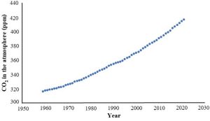
At this point it would be fair to wonder: hang on, just how do we know about carbon dioxide levels from the past? The answer is, we combine evidence from direct and indirect measurements. The first type is relatively straight forward. Researchers at a site near Mauna Lau, Hawaii (U.S.A) have directly collected and analyzed air samples since 1958. That work is ongoing and has produced one of the most famous (as these things go) graphs to be produced by scientists (Figure 14.19).
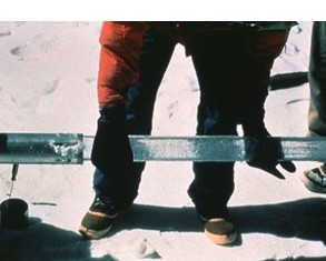
The second type of data collection is more complicated than the first and involves indirect measurements (also called proxy measurements) to give us information for the years before we sampled the atmosphere in real time (i.e., prior to 1958). Proxy measurements utilize samples of ancient atmospheres that have been trapped in bodies of ice, glaciers, that persist for hundreds of thousands of years. Very briefly, long cylindrical vertical cores are taken from thick sections of glaciers, and air in pores from thin sections is analyzed to determine concentrations of CO2 and other gases in them (Figure 14.20).
From here, we make two assumptions. First, it has been well-established that a glacier gets older with depth. Plus, we can use various tools of geology and chemistry to establish the age, in years, of different layers of ice. Second, air in the bubbles we find today are tiny samples of Earth’s atmosphere from the past—they represent a series of snapshots, of sorts, of the air that must have been present when the ice formed. By combining age data with chemical analyses we can reconstruct the history of the composition of the atmosphere (Figure 14.21).
We will return to the topic of CO2, including the long-term trends in its atmospheric concentration, shortly.
Methane. Emissions to and concentrations of CH4 in the atmosphere are far lower than those for carbon dioxide, but this gas is a much more powerful GHG: one molecule of methane contributes as much to global warming as about 24 molecules of carbon dioxide (i.e., it has a GWP of 24 CO2). What are the sources of methane? As with CO2, both natural and anthropogenic processes release CH4 to the atmosphere. This gas is produced during anaerobic decomposition of organic carbon compounds in swamps and other natural low-oxygen environments (Chapter 4). It is also released from the digestive systems of animals such as cows, camels, elk, and termites. In those cases involving animals, mutualism between a larger organism and microorganisms living inside of it is responsible for digestion of plant material, survival of both participants, and production of methane. The worldwide breeding of billions of dairy and beef cattle by farmers adds a substantial amount of CH4 to the atmosphere (see Chapter 9), an activity that is likely to increase as both the number and standards of living of humans go up (Chapter 8). Burning of fossil fuels, deforestation, and landfills, also linked to increasing resource use by people, produce methane as well. Methane is the second-most-important anthropogenic GHG by quantity, accounting for approximately 15% of our emissions[13]. Several phenomena reduce the amount of methane in the atmosphere (i.e., are sinks). For instance, certain specialized bacteria convert it into CO2 as part of their normal metabolism. In Chapter 13 we saw that combustion of methane produced in landfills is similarly transformed. Yes, carbon dioxide is still a greenhouse gas, but since it is a far less effective GHG than methane, we generally view these reactions as beneficial (in terms of effect on greenhouse warming). Overall, though, processes that remove methane cannot keep up with inputs of the gas, so it continues to accumulate. Like those for CO2, atmospheric concentrations of CH4 have gone up precipitously in recent centuries: today’s levels are more than twice as high as those from the preindustrial age (again, as indicated by analyses of glaciers and direct measurements). Data suggest that the rate of increase has accelerated in recent years[14].
Nitrous oxide. The atmospheric concentration of this gas, N2O, is considerably lower than that of either CO2 or CH4, but it has a GWP of approximately 3007. A little more than half of it enters the atmosphere from natural cycling of nitrogen (Chapter 4). Agriculture is responsible for the bulk of anthropogenic nitrous oxide, with fuel combustion and industrial processes making contributions as well. All told, N2O is the third highest GHG on the list[15]. Chemical reactions convert it to other gases, but since its concentration is going up, those sinks do not currently keep pace with sources. Also of interest is the role nitrous oxide plays in ozone depletion, the second global-scale air pollution issue we will consider (below).
Fluorinated and chlorinated gases. This broad group includes several manufactured compounds that consist of fluorine (Fl), chlorine (Cl), carbon, and other atoms in various combinations. These days, emissions of fluorinated gases far outpace those of chlorinated gases because the latter have been largely phased out of production and use (more can be found below, including figures of them, in the discussion of ozone depletion). The relative concentrations of these are very low, yet they still can make a substantial contribution to warming because they are at least 10,000 fold more potent as greenhouse gases than carbon dioxide (sulfur hexafluoride, SF6, tops the list with a GWP of 22,500[16]). Another very important consideration is that the residence time of these gases in the atmosphere tends to be very long, likely thousands of years in some cases. Note that no natural source produces any relevant amount of these types of gases, even if natural processes can remove them from the atmosphere (more shortly).
Carbon dioxide is linked to fossil fuel combustion: a closer look
A balance between natural inputs and outputs meant that concentrations of CO2 in the atmosphere remained constant during much of the past thousand years. However, anthropogenic activity—notably, the burning of coal, oil, and natural gas—since the start of the Industrial Revolution has disrupted that long-held equilibrium: the organic carbon that had been stored in the lithosphere as fossil fuels for millions of years was converted to CO2 and began moving into, and accumulating in, the atmosphere (Chapter 10). Keep in mind that a measurable increase in the concentrations of atmospheric GHGs is of concern because more outgoing heat energy is absorbed and re-emitted toward Earth (i.e., the greenhouse effect is enhanced). The planet’s surface then gets even warmer than it was in the presence of a natural greenhouse effect. In other words, the start of the upward trend in average temperature we noted at the beginning of this discussion—and which we are trying to answer in question #2—coincided with industrialization, and industrialization resulted in increased emissions and atmospheric concentrations of CO2. These links between human activity and changes in atmospheric chemistry are crucial pieces of evidence used to both explain what we have seen during the past 150 or so years and predict what is likely to happen in the future. Most of this discussion is centered on carbon dioxide, although the concentration of methane followed a similar trend since the 1800s. Due to differences in patterns of human activities and emissions, nitrous oxide and fluorinated / chlorinated gases did not begin to increase until the 1960s.
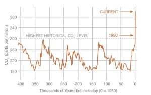
Atmospheric concentrations of some GHGs are higher now than in 800,000 years
Using ice core analyses, scientists have reconstructed the 800,000-year history of atmospheric carbon dioxide and methane. The concentration of each gas is higher now than at any time during that long period for which we can collect data. We will see a graphical representation of that trend shortly.
GHG concentrations have been linked to temperatures in the past
As we learned above, rising concentrations of gases like CO2 are of concern on their own because of their chemical properties: as GHGs accumulate in the atmosphere, more heat will be re-emitted to Earth’s surface. Scientists have also noted compelling evidence from ice-core data of a close link between temperature and atmospheric greenhouse gas concentrations during the past 800,000 years. Using chemical analysis of certain atoms present in glaciers, a timeline of past temperatures has been reconstructed and it follows the same trend as those for CO2 (Figure 14.22.a).
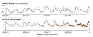
If we assume the rules governing the universe have not changed with time, we should expect that the relationship between GHGs and temperature is the same today as it was historically. The temperature-CO2 link since 1880 is evident as well (Figure 14.22.b).
Question #3: If the answer to #1 is yes, then what would be the consequences? Continuing the list of questions started a while ago, we now ask: who cares if the temperature goes up by a few degrees? Does it really matter? Well, we noted earlier that the biggest risk of global warming is not that things will be noticeably warmer everywhere, but that climates will be affected in various and, in some cases, profound, ways. Since organisms are connected to and shaped by their environments (as explored multiple times in this book), all members of the biosphere, including humans, could be adversely affected by climate change.
Changes in precipitation patterns
Temperature influences the movement of water among Earth’s reservoirs in two important ways. First, global warming heats the oceans and drives more evaporation into the atmosphere (as noted earlier, more water vapor leads to more warming and subsequent evaporation). Second, rates of condensation of water from air decline as temperature of the air goes up; in essence, warmer air carries more water than does cooler air. Researchers expect that these changes to the atmosphere will bring about higher rates of precipitation in some places while some areas will get drier during the next several decades. In the United States, for example, increased volumes and rates of rainfall have already been noted in northeastern regions, whereas droughts have gotten worse in some southwestern regions[17]. Organisms adapted to precipitation patterns in their current natural environments would undergo stress and possible extinction, but the consequences of shifting rainfall to humans could be profound as well. Among the worries facing many of the world’s peoples are: flooding and other extreme events would cause loss of life, property, and agricultural production. Scarcity of resources like clean water, habitable land, and food could then lead to increased conflicts among states and nations.
Rising sea level
Water expands as it is heated. So, even without additions, water in the oceans will simply take up more space—that is, thermal expansion will cause it to rise and encroach further onto land—as global temperatures go up. More water is introduced as well, though, when glacial melt (more below) flows into the oceans. Taken together, these two phenomena have driven sea level to increase by approximately 22 cm, or 8 inches, since 1880[18]. Worth noting, though, is the way the rate of increase has accelerated in recent decades. For most of the 20th Century, it was about 1.4 millimeters per year but rose to 3.6 mm per year between 2006 and 2015. Scientists project that the surface of the world’s oceans will continue to rise by at least one meter throughout the rest of this century (estimates range from 0.2 to more than 2.0 m). Natural ecosystems, particularly those at delicate water-land interfaces, are sensitive to such rapid and dramatic change, and extinctions of species living in specialized habitats are possible. Since roughly one third of the world’s peoples live within 100 km of a coastline[19], even a modest rise would also disrupt human structures, systems, and lives. Cities such as New York, Washington, Miami, New Orleans, Los Angeles (all U.S.A.), Tokyo (Japan), Venice (Italy), Mumbai (India), and Shanghai (China,) as well as areas within many nations in Asia, Africa, and South America are at risk. The Maldives (Indian Ocean) is a small, low-lying island nation made famous in part because it could be completely inundated by 2100 if sea level continues to rise (Figure 14.23).

The relevance of severe flooding surely is obvious: death, damage, and destruction are all likely. However, you should keep in mind that many people find themselves increasingly plagued by low-impact events. Among other trouble caused by this nuisance flooding is heightened vulnerability to extreme storms. The frequent presence of excess water can make losses due to, say, a hurricane, even worse[20]. Also note that stagnant flood waters are ideal environments for reproduction of disease-carrying mosquitoes.
Changes in ocean circulation
Water mixes and moves among Earth’s oceans via a complex mechanism called the global conveyor belt (Figure 14.24).
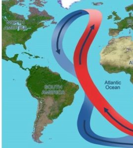
Briefly, water sinks or rises due to temperature and salinity variations, and these vertical displacements ultimately drive the lateral circulation of massive volumes of water from cold to warm regions (and back again). Among other important outcomes it produces, the conveyor belt moves heated equatorial water to the northern Atlantic Ocean, making The United Kingdom and other parts of Europe much warmer than they would be otherwise. A combination of changing precipitation patterns and melting glaciers would introduce more freshwater into the oceans, disrupt the current cycle of rising and falling water, and ultimately slow circulation. A weakened conveyor would cool affected areas—perhaps by a great deal—providing one example of the way general warming of the Earth would bring about a range of location-specific effects.
Melting of glaciers
Like the many other systems we have considered, the relationship between inputs and outputs—in this case, the freezing of water and the melting of ice, respectively—controls the amount of material inside the glacier at any time. As average global temperatures have risen, rates of melting have outpaced rates of freezing, and that imbalance seems to be increasing. Ground-based photography has shown that many glaciers around the world have gotten appreciably smaller during the past century (Figure 14.25), and recent data collected from satellite images indicate about 400 billion metric tons in annual net ice losses[21] from those in Greenland and Antarctica—which together contain about 99% of Earth’s ice—since 2002[22],[23].
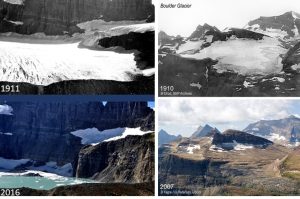
Glacial melting is important for at least three reasons. First, the water it releases contributes to rising sea levels. In fact, contributions from meltwaters relative to that of the thermal expansion of water (described above) is thought to be greater now than it was just a decade ago because of accelerating rates of melting[24] (note that melting sea ice does not contribute to these rises—the water is already in the ocean, albeit in solid form). Second, it slows the global conveyor belt (above) because it introduces freshwater into oceans and reduces salinity. Third, areas that depend on water released from melting glaciers to recharge depleted groundwater and other reservoirs (Chapter 11) face water shortages as the amount of water stored in ice dwindles each year.
Ocean acidification
Although not directly linked to global warming, this outcome is related because it is caused by increased CO2 in the atmosphere. Put simply, excess carbon dioxide accumulates and alters atmospheric chemistry as we have noted. Some of it moves into the hydrosphere, though. Once in the oceans, it combines with water and a naturally occurring ion called carbonate (CO32-) to produce bicarbonate (HCO3–). This reaction has lowered ocean pH by 0.1 unit (review Box 14.1, above), or, in more meaningful terms, increased acidity by 30%. Marine organisms needing carbonate to build shells (e.g., clams, corals, sea urchins) struggle to succeed in their changed environment[25]. If the rise of atmospheric carbon dioxide continues its current trajectory, acidity will increase by 150% by the year 2100[26][/footnote]. Shifts in ecosystem structure are likely as organisms adapted to current pH levels would face increasingly hostile conditions. People who rely on marine resources for food and income would also be adversely affected.
Changes to global primary production?
Climate change could reduce the number of marine phytoplankton, the largest source of fixed C and gaseous O2 on Earth. Recent data indicate declines in both the size and success of the communities of these critical organisms. If this trend continues, not only would ocean ecosystems suffer damage, all aerobic organisms (including humans) would be imperiled [27].
Altered disease distribution?
We know that changes in the physical, chemical, and biological properties of an environment can influence all biological entities present in an ecosystem, including those that cause diseases (i.e., pathogens). So, higher average temperatures have the potential to change the distribution of human parasites. Malaria, for example, is generally confined to tropical and subtropical regions because both the protozoan that causes it and the mosquito that transmits the protozoan to people require relatively warm and wet conditions. If temperatures rise, though, the ranges of this and other important diseases could increase and affect northern countries. Additional research is needed before definitive conclusions can be drawn.
An increase in both the intensity and number of storms and fires
Many climate scientists have suggested that since hurricanes gather energy from the ocean, they will strengthen as water temperature rises. Furthermore, some already dry areas—like those in western portions of the U.S.—will become increasingly subject to wildfires as droughts worsen. Further research is needed to sort out the validities of these prediction, but they are plausible and even seem to be supported by recent events (i.e., unusually large and devastating wildfires).
Rapid, dramatic changes
We should make a final note about these and any other potential adverse consequences of warming and climate change. Given the myriad interactions and complexities in the system, a growing number of researchers express concern that the rate of some changes could greatly accelerate if Earth reaches what is often called a tipping point, a critical level at which a cascade of events is initiated. So, although atmospheric carbon dioxide might continue to rise at a constant rate for an extended period, it could reach a concentration that causes sudden and unexpected shifts in temperature, precipitation, ecosystem distribution, or biodiversity. Once change occurs, it would then be very difficult to return an affected system to its former conditions. It is somewhat akin to people shuffling slowly and steadily toward the edge of a cliff. At the edge, just a few centimeters of horizontal movement results in hundreds of meters of vertical travel as they suddenly plummet to a low elevation.
Question #4: If the answer to #1 is yes, then what can we do about it? Finally, we get to our last question. Since evidence increasingly points to human activity, notably greenhouse gas emissions, as the primary cause of global warming, we have the power to affect it. Simply put, if we can bring rates of inputs and outputs of GHGs back into balance, we could stop further warming and climate change and perhaps even reverse what has already occurred. Some possible solutions are listed here. Keep in mind that no single strategy would solve the problem, rather a combination of ideas and approaches will very likely be needed. Here are some ideas likely to be most effective.
Reduce GHG emissions
Carbon dioxide. Since this is the single most important anthropogenic greenhouse gas, it will receive the bulk of our attention. Of the many steps people could take, we will consider three having the greatest potential to slow the accumulation of CO2 in the atmosphere. First, decreasing the amount of coal, oil, and natural gas burned to generate electricity and power transportation—that is, accomplishing the same amount of work with less combustion—would lower carbon emissions. Improved efficiency of air conditioners, refrigerators, and other appliances, along with better fuel economy for motor vehicles, are some of the ways reduced fossil fuel usage is accomplished. For instance, the tightening of federally mandated fuel efficiency standards for automobiles sold in the United States has lowered the use of gasoline to a degree. Ultimately, though, a substantial switch away from fossil fuels to energy sources like wind, solar, and hydroelectric that do not lead to emissions of CO2 will likely be needed to effectively combat the problem of global warming (we will return to this point below). Exhaustive coverage of the economic, cultural, and scientific issues that limit the ambition, rigor, and effectiveness of such measures is not possible in this space. Suffice it to say that enacting relevant laws is enormously difficult because of multiple disagreements and competing priorities among interested parties. Second, managing expectations of ever-higher standards of living—that is, encouraging less consumption of goods, services, and transportation that rely heavily on fossil fuels—would reduce emissions of carbon dioxide. Finally, more use of agricultural practices that minimize decomposition of soil organic matter would reduce an important source of CO2.
Methane and nitrous oxide. Better agricultural practices and management of waste, as we saw earlier in this chapter, limit the amount of these gases reaching the atmosphere.
Others. Stricter regulations and monitoring of the powerful synthetic GHGs noted earlier (fluorinated and chlorinated gases) through recycling, the use of alternative compounds, and careful control to limit releases, all lessen their ability to increase Earth’s greenhouse effect.
Sequester carbon dioxide
A combination of technology may be used to pull CO2 from smokestacks and other sources before it moves into the atmosphere. After its capture, the carbon dioxide can be stored in the lithosphere or other places (a practice called carbon capture and storage, CCS) thus reducing the rate of inputs of the gas to the atmosphere. A related strategy, carbon capture and utilization (CCU), makes use of the carbon dioxide in the manufacturing of plastics and other products (under the proper conditions, CO2 can be combined with other chemicals to build useable solid materials). Although CCU currently operates on a small scale, it has the potential to dramatically reduce the net amount of carbon in the atmosphere and reduce the problems of plastic pollution. Research on both CCS and CCU continues[28].
Slow or reverse deforestation
Reducing rates of deforestation would affect both inputs and outputs of atmospheric CO2. The burning of trees—a typical approach when large, forested areas are cleared—is an important GHG source because it converts stored organic carbon into carbon dioxide. The sink side of the equation is influenced in that fewer trees and other photosynthesizing organisms would draw carbon dioxide out of the atmosphere. In short, land clearing for agriculture, housing, or forestry increases the movement of carbon from the biosphere to the atmosphere while simultaneously decreasing the movement in the opposite direction. Actively increasing the number of trees is another piece of this solution, although afforestation would conflict with other land uses to support a growing population.
Adapt to a changed world
What if we do not take the steps needed to address global warming? Some people already have given up, concluding that nothing can be done in any case, are in denial that change will occur, or believe it is natural and inevitable. How might we diminish the adverse consequences and live with climate change?
Build protective structures. As oceans rise, flood risks in low-lying areas increase. Venice (Italy), for example, has contended with sinking land for many centuries, but it could become uninhabitable within a hundred years if sea level changes as predicted. Many other coastal zones are threatened by rising water, and the problem is likely to get worse in coming decades. What can be done? In addition to relocating millions of people to higher ground, bigger, stronger, and more expensive levees, sea walls, and dams could be built to protect the most vulnerable areas. These structures would need to be designed to hold back ever-more-powerful storm surges, one of the possible outcomes of global warming. In other words, big investments would be required to avoid the kind of damage seen in 2005 when Hurricane Katrina overwhelmed inadequate levees intended to protect New Orleans, Louisiana (U.S.A.), a city that already sits below sea level[29].
Restore beaches. As coastal residents know, sandy beaches are far from static. Even in a relatively uneventful year, they move and change shape due to multiple natural forces. Resort communities that rely on summer tourism therefore invest considerable amounts of money to replace lost sand and maintain attractive beaches indefinitely. If oceans rise and hurricanes become more intense, beach maintenance and restoration will become increasingly difficult and expensive.
Relocate affected people. Even if we can build structures or otherwise modify environments to protect them from the effects of climate change, certain places are likely to undergo irreparable damage. Simply put, some people will be forced to permanently move elsewhere. The number affected is hard to predict with certainty, but since about a third of the world’s population lives near a coastline[30], many hundreds of millions could potentially be displaced. It is unclear where they would go and how the enormous cost associated with their relocation would be met.
Manage food shortages, diseases, and conflicts. We will not reiterate what was said above about these consequences, but they all should be added to the list of necessary adjustments if people elect inaction and adaptation in favor of prevention and reversal of climate change.
Coordinating a global response
The solutions proposed here have been difficult to implement for many reasons, including the fact that climate change is a global-level concern that requires global-level strategies to be mitigated. In other words, peoples and countries with very different levels of influence, wealth, and attitudes need to coordinate their efforts. Understating matters by a fair amount, it has not been easy for the world’s nations to come up with an effective plan palatable to everybody. Two groups trying to manage scientific research as well as appropriate action are very briefly described here.
Intergovernmental Panel on Climate Change (IPCC). This is an international group working through the U.N. to monitor and summarize the current state of the science of climate change research. It has issued five formal statements during its roughly three-decade existence (one every six or so years) that provide predictions and recommended actions based on the available data. It has been a very important and influential organization and continues to gather, interpret, and disseminate the evidence related to human-caused climate change. You are encouraged to explore the work of the IPCC, including its latest report online[31].
United Nations Framework Convention on Climate Change (UNFCCC). Established in 1992, this organization is designed to help member countries study and reduce anthropogenic contributions to climate change (consult its website for more information[32]. The Kyoto Protocol (1994) and the Paris Agreement (2016) are two major initiatives of the UNFCCC to limit greenhouse gas emissions. Efforts to reach their stated goals have been hampered by several obstacles, however. Notably, developing and developed nations are motivated by different priorities and notions of fairness and justice. Countries like the United States, currently responsible for about 25% of the CO2 put into the atmosphere, disagree with countries such as China, which are likely to emit far more of this and other greenhouse gases in the future, on what is the most equitable way to move forward. A nation like The Maldives (described above), argues that, although it contributes relatively little to the problem, it bears a disproportionate amount of the burden of climate change. Arguments about the economic consequences of any proposals also tend to limit their scope and effectiveness. Moreover, the fact that some people do not accept the science of climate change, a topic we will revisit shortly, adds to the difficulties of implementing appropriate responses.
Evidence-based predictions
Careful analysis of data enables scientists to describe the history of Earth’s climate during the past few centuries. Now, though, we must ask: what about the future? This critical question is the subject of continued study.
Using computer models. Computer models are employed to help predict what will occur in coming years. In simple terms, data about climate such as current temperatures, ice cover, cloud cover, and greenhouse gas emissions, are inputs to a computer program and forecasts about temperatures, rainfall distribution, sea level, and other concerns are outputs. These programs themselves are designed to account for as many variables as possible as well as the multiple and complex interactions among all the relevant parts of the system. Although models differ in the specific outputs they produce, most point to a warmer planet overall—as stated previously, on average, the increase will likely be 1.1 – 5.4 ºC by the end of this century. Models also quantify how much sea level will rise (0.2 – 2.0 m) and weigh in on the other consequences described above.
Challenges to modelling the future. A model is only as good at predicting the future as is the validity of its inputs and assumptions. Thus, as our understanding of Earth’s climate systems improves, so does the quality of our models. Several challenges still limit the reliability of models.
The role of feedback
Recall from Chapter 2 that feedback can either accentuate or attenuate a system response, leading to change or stability, respectively. Some unanswered questions about the role feedback will play in climate change hamper, somewhat, the validity of models.
Positive. Here, past increases in greenhouse gas concentrations, higher temperatures, shifting precipitation, melting glaciers, and sea level rises get amplified by current and future system responses; in other words, the rate of climate change increases. Two relevant examples illustrate this type of feedback. First, as glaciers melt and get smaller, they shrink faster and faster. When they are very large, their light-colored ice and snow reflects most of the incoming light energy, that is, they tend to raise Earth’s albedo. As temperatures go up, the melting ice reveals the dark-colored rocks and soil that were beneath, leading to lower albedo. More energy absorption, in turn, increases temperature and accelerates future melting (Figure 14.26; compare to Figure 2.10).

Second, since evaporation is driven by temperature, more and more water is converted from liquid to gas as oceans warm. The addition of water vapor to the atmosphere then increases the amount of infrared energy emitted back to the surface, leading to even higher temperatures and rates of evaporation in the future. As we have seen repeatedly: current change accelerates future change. Models give varying weight to positive feedback as our understanding of it evolves.
Negative. Past outputs are essentially cancelled out by current outputs in this case, and temperature and climate remain stable. Again, we refer to two important examples. The first involves the response of primary producers to increased levels of carbon dioxide in the atmosphere. We might expect that carbon fixers like plants and algae would be stimulated to grow as more C is added to their environments, and this increase in primary production would then draw more CO2 out of the atmosphere. So, Earth’s system would remain stable: it would respond to more of this important GHG by increasing the size of the living C sink. Unfortunately, this proposed feedback mechanism probably contributes little to stability. Keep in mind that carbon is generally not the limiting factor for primary producers, rather, lack of nutrients such as nitrogen, phosphorous, or iron tends to slow their growth before carbon is exhausted; environmental changes like loss of topsoil are also more important (see Chapter 9 for more about limiting factors). Furthermore, some research even suggests that excess CO2 might slow the growth of plants, therefore reducing rates of fixation. Our second example of negative feedback returns to the way increased temperature leads to more evaporation. Unlike its role in positive feedback noted above, though, water vapor driven from heated oceans would adhere to dust particles in the atmosphere and form more clouds. This increase in cloud cover would block more incoming light energy—that is, albedo would be higher—and Earth’s average temperature would ultimately decrease. Many climate models incorporate changes in cloud cover, but the extent to which this variable will affect future trends is not entirely understood.
Which type dominates? Each of the four examples of feedback just described, along with several others, is surely active to some extent. However, given the observed continuing measurable increases in atmospheric CO2, average temperature, and sea level (as well as the higher rates at which they have changed in recent decades) positive feedback seems to be dominant. Negative feedback may be slowing the rate of climate change but its power to bring stability is clearly limited.
The complexity of Earth’s systems
The system under consideration—which includes the atmosphere, hydrosphere, lithosphere, and biosphere—is characterized by enormous size and complexity. Although we have learned much, our understanding of the interactions and factors affecting climate is certainly incomplete and continues to evolve.
Unknowns about future human behavior
The predictions about temperature and sea level noted above are expressed as ranges in large part because we simply cannot predict with certainty what humans will be doing during the coming decades. Will greenhouse gas emissions increase? Decrease? Remain the same? Arguments can be made for each of those possibilities, and they depend on future population growth, standards of living, dominant agricultural techniques employed, fossil vs. non-carbon fuel usage, and extent and rates of deforestation. Only with time will we know the answers for sure.
Measurement uncertainty
Scientists use multiple tools and instruments to measure, among other properties, temperature and chemical composition of Earth’s complex atmosphere. Many readings need to be taken at different locations, altitudes, and times, instruments must be carefully maintained and calibrated, and scientists must be consistent and well trained. So, as in all research, measurement uncertainty is acknowledged, quantified, and considered when predictions are made.
Testing the reliability of models. How do we know if a computer model can be trusted? A climate model can be tested, or validated, if we input data from the past, say 300 years ago, and then see how well the output predicts what we know to be the current state of the climate (i.e., according to the computer, what will happen in the future). Since we assume the rules governing the behavior of Earth’s climate systems do not change with time, a model that accurately describes what happened during the previous centuries will likely be equally successful predicting the century that is yet to come. It turns out that some models are better than others, but none is 100% reliable. Interestingly, a common problem is that evolving models underestimate how much warmer things will be: attempts at validation indicate that temperature should be lower than it really is, indicating that changes could be more severe than we expect.
Climate change doubters and deniers: who and why?
Even as evidence for its causes and consequences mounts, some people deny the reality of climate change.
Degrees of denial. It is fair to say that climate-change denial is generally not a yes-or-no question but that most people find themselves somewhere on a spectrum from complete denial to complete acceptance. Some people refuse to believe that any warming or other changes have even occurred, despite evidence to the contrary. Some recognize that data about increases in greenhouse gases and temperature are convincing but maintain there is insufficient evidence to link the observed changes to human actions. Importantly, they tend to argue that we should wait to take any steps intended to combat climate change until the science is stronger. Still others accept that climate change is caused at least in part by humans but that the processes cannot be reversed. In other words, they see our only option is adaptation to a changed world. Finally, some people, including most scientists, are persuaded by the evidence and accept that human-induced climate change is a reality that can be at least partially mitigated. They often hold the view that, although more needs to be learned about the science of the problem, the data are sufficiently compelling to justify making proactive changes immediately, even some that might be very inconvenient.
Who are the deniers?. Just who denies and who accepts the science of climate change? Lumping together all the doubters mentioned above into one heterogenous group, numerous estimates suggest that just 3% of experts—that is, climate scientists—do not accept that human emissions of GHGs are affecting the greenhouse effect and driving climate change[33]. A somewhat larger percentage of people without expertise in science (the number likely ranges between 10 and 50%) doubt at least some of the science of climate change. Put another way, knowledge of the scientific method and data analysis tends to be an important factor determining where one lies on the denial spectrum.
Sources of doubt. The reasons people cite for their doubt and denial are numerous. Some draw upon the science of climate change—often misrepresenting or misunderstanding the meaning of the data—but many are rooted in values, opinions, or other non-scientific arguments. Although strong and objective data generally move scientists, many other people, including lawmakers and members of the public, are not so easily swayed by even the most compelling evidence. Convincing skeptics is challenging, but not impossible: see the essay in Box 14.3 by guest writer and former member of the U.S. House of Representatives Robert Inglis (Republican from South Carolina) for one example of the power of science to change minds.
Box 14.3. Evidence changed my mind: a note from Robert Inglis, former member of U.S. House of Representatives
During my first six years in the U.S. Congress (1993–1999) I said that climate change was nonsense, a figment of Al Gore’s imagination. I represented a very conservative district in South Carolina, and I spouted the party line. Then, after being out of Congress for six years, I had the opportunity to run again for the same seat in 2004. My son challenged me to care about the environment. I got re-elected and went to Antarctica with the House Science Committee and saw the evidence in the ice core drillings. On another Science Committee trip at the Great Barrier Reef I was inspired by the faith of an Aussie climate scientist named Scott Heron. I wanted to be like Scott, loving God and loving people, so I came home and introduced into Congress a revenue-neutral, border-adjustable carbon tax. My political timing wasn’t so good as the Great Recession was on. I got tossed out of Congress in a Republican primary in 2010 for various heresies against the temporary Republican orthodoxy, the most enduring of which was my willingness to continue to say that climate change is real. Ever since I’ve been out to convince fellow conservatives that it’s actually quite conservative to care about climate change. I founded and direct a grassroots educational campaign that we’ve branded as republicEn.org.
My advice to students and members of the public at large is this: when factual observations overtake our shaky ideologies, it’s better to be overtaken.
–Bob Inglis, 2019
Here is a short list of some common sources of doubt, along with brief responses and clarifications.
Natural sources of carbon dioxide outweigh anthropogenic ones
We learned earlier that anthropogenic sources contribute about 10% of the CO2 that enters the atmosphere annually. Some people have used these data to suggest that humans play an insignificant role in the cycling of this important greenhouse gas. However, that relatively small amount has thrown off the equilibrium between sinks and sources that was in place for many centuries prior to 1880. The yearly surplus from fossil fuel combustion and other activities accumulates, driving the atmospheric concentration of carbon dioxide higher and higher (review Figure 14.19).
But….water vapor comes from natural sources!
Water vapor is the most important greenhouse gas, accounting for most of Earth’s greenhouse warming. It is also largely produced by natural processes. So, the argument often goes, observed changes in temperature cannot be linked to human emissions of carbon dioxide—they are simply trivial in comparison to this natural GHG. As is stated in the above point, though, human contributions have shifted a long-standing balance between sources and sinks of several greenhouse gases. Yes, water is more abundant and more important, but that hardly means increasing levels of CO2 are therefore irrelevant: as we know, temperatures started to rise only after the widespread burning of fossil fuels by humans. We need to also remember that warming caused by carbon dioxide and other anthropogenic GHGs increases the rate of evaporation and the amount of gaseous water moving into the atmosphere. In other words, human activity does indeed affect the water cycle.
Fluctuations in temperature and other climatic factors are normal and natural
This statement is supported by scientific evidence: Earth’s long history has been characterized by many changes to its average temperature and climate. The rapid pace at which current changes are occurring, though—including the high rate of GHG accumulation in the atmosphere—appears to be unprecedented.
Lower sunspot activity will cool Earth in the coming decades
Some people—including a small number of scientists—believe the Earth is actually cooling and that any upward pressure on temperature will be cancelled out by larger climate forces in the near future. An important piece of evidence used to support this hypothesis is the prolonged period of low sunspot activity and coincident cooling that occurred during the 17th Century. The so-called Little Ice Age (review Figure 14.14, above) was characterized by lower average temperatures for several decades, but most scientists hold that the reduced solar activity during the same period was not the only factor at work and would have been insufficient to account for all the observed climate change in any case. Major volcanic eruptions likely had a significant impact, for example. Other problems limit the plausibility of this cooling effect. First and arguably foremost, we have not learned how to predict future solar output, only record what has already occurred. In short, we really have no idea what will happen to sunspot activity in the short or long run. Secondly, the fact that Earth’s temperature has risen steadily since 1880, despite several changes in energy output from the sun in the past century, suggests other forces must make a larger contribution to global warming.
If we can’t forecast tomorrow’s weather, how can we predict next century’s climate[34]?
Frustration with inaccurate weather forecasts is used by many to dismiss the science of climate change as altogether unreliable. It turns out, though, that “weather” and “climate” refer to distinct phenomena, with the former being harder to predict than the latter. Weather is made up of short-term conditions such as temperature, humidity, rainfall, and wind and is highly variable from day to day. Climate, on the other hand, includes long-term characteristics prevalent in a region such as the range of temperature and total rainfall in a given year. In short, the weather conditions at any time are a function of the climate of an area. January snow in a place like upstate New York (U.S.A.), for example, is hardly surprising because its climate is appropriate for such events. So, what does this have to do with the reliability—or lack thereof—of predictions? Weather forecasting is particularly difficult because it tries to describe details about the timing and severity of properties like upcoming precipitation and temperature. “Will it rain Tuesday?” is the kind of question a weather forecaster tries to answer by providing probabilities (“70% chance of showers”, and the like). Since so many forces and interactions influence specific weather over the course of just a few days, we do not always get it right. Alternatively, climate projections aim to describe trends that will happen in the long run. We know, for example, that regular shifts in the tilt of this planet bring spring and melting of the snow in upstate New York and cause winter to return by November or so. Changes unfolding during many years can only be detected with long-range, persistent monitoring, and might be temporarily obscured somewhat by today’s weather events. As computer models become increasingly accurate in their ability to take past data and predict current conditions (i.e., they can be validated as described above), our confidence in predictions of future climates grows. But you should still consider packing an umbrella just in case tomorrow’s forecast for “10% chance of showers” turns out to underestimate the likelihood of rain.
How can global warming be real when this winter was so cold?
Our succinct answer to arguments like this one is: climate change refers to long-term global trends, not what occurs in a location during a single month, season, or year. So, an unusual snowstorm in May, for instance, is not evidence of anything in particular except that weather can vary from year to year. It certainly does not invalidate more than a century of data on increased temperature and sea level rise. People’s misconceptions about the meaning and relevance of climate change are not surprising, though, because “global warming” seems like it ought to lead to warmer weather everywhere. And, deniers tend to seize upon isolated facts to support their world views—the same people who claim that a warm February debunks the science of climate change are generally silent on the possible significance of an unusually hot October (again, neither anomaly should be cited to support any hypothesis).
The economic consequences of change would be too severe
This common view reflects some uneasiness about the steps we need to take, but it in no way invalidates the science of climate change. That is, although the consequences of reducing GHG emissions may indeed be inconvenient and difficult, it is illogical to conclude that global warming is therefore something we can dismiss as fiction. It is also by no means certain that changing from non-renewable fuels like coal and gasoline to renewable sources such as solar and wind would lead to economic hardship. Yes, a conversion to a non-carbon economy, with all the necessary modifications to infrastructure, transportation, agriculture, and so on, would not be easy to manage and would likely cause some short-term pain. However, the development of new renewable energy technology would offer new investment opportunities, encourage innovation and entrepreneurship, and provide long-lasting economic, military, and public-health security.
We do not know enough to justify making changes
Briefly, those that worry about the social and economic costs of reducing greenhouse gas emissions often argue that the science is still too uncertain to justify plunging the world into the dramatic changes that would result from a move away from fossil fuels. Again, financial disaster would not necessarily be the outcome in any case—like environmental science, economic forecasting is itself plagued by uncertainty. In somewhat oversimplified terms, it comes down to a conflict between those who think we should wait for more science before doing anything and those who do not want to risk waiting any longer to respond to the threat of climate change despite lingering uncertainties and some unanswered scientific questions.
We cannot do anything about it anyway
There are some who either think global climate change is entirely the result of natural forces beyond our control or is a problem that has already gone too far for us to remedy. We have addressed the first argument once before. As to the second, current climate forecasting considers various scenarios based on different anthropogenic GHG emissions during the coming decades and concludes that we still have an ability to slow warming if we take steps now. Most climate scientists acknowledge that some additional warming is inevitable at this point—something like 2 ºC within a hundred years—but predict it will be much more severe—up to 6 ºC during the same timeframe—if we do nothing.
Other, non-scientific, objections
Many other arguments having nothing to do with objective science, those based in values, beliefs, opinions, and attitudes, also underlie denial and skepticism about the reality of climate change. These are often deeply entrenched and difficult to overcome. For example, it is very hard to convince people that the data and evidence supporting conclusions about climate change should be taken seriously if they believe scientists are inherently unethical or assume the whole story is a hoax perpetrated by the news media.
Denial matters. The solutions to human-caused climate change have been very difficult to implement for many reasons. Although the steps needed are seemingly straight forward, that is, greatly reduce GHG emissions, getting to an economy based on non-carbon fuels is of course not at all easy and requires people to make some tough choices. Vocal and influential deniers of the evidence-based conclusions of scientists make the necessary policy changes that much harder to bring about because they cast doubt on the notion that the short-term challenges are truly worth the effort.
Now what?
Acknowledging information gaps and uncertainty, data strongly indicate human activities have increased Earth’s average temperature and brought about climate change. Whether the resultant adverse consequences listed above come to pass tomorrow depend on choices made by us today.
14.2.4. Ozone depletion
Our second global-level concern does not get as much attention as global warming these days, but it is still quite relevant. Here we briefly explore the causes, consequences, and remediation of this nuanced and complex problem.
First things first: “ozone depletion” and “global warming” are not synonymous!
Despite what is widely believed, these two global-level air pollution issues are not the same. As we just learned, warming is caused by the accumulation of greenhouse gases and is linked to climate change, rising sea levels, and many other consequences. This second problem involves the loss of an important atmospheric gas, ozone. Depletion of ozone results from different mechanisms than does climate change, and the adverse effects of these two phenomena are distinct. Most importantly, ozone depletion should not be understood to be the primary cause of global warming.
A second clarification: it is not really a hole.
We should also address a second misconception before we get to the details of this topic. Although the term “ozone hole” is often used to describe ozone depletion, it is not the best way to visualize the situation. As we will learn shortly, depletion refers to a decline in the amount of stratospheric ozone over a given region of the Earth’s surface, not an actual opening in which zero ozone is present. This clarification should not be read as an attempt to minimize the urgency of this problem, because a reduction in ozone levels can lead to serious, in some cases even deadly, outcomes.
Ozone gas: the essentials
Our discussion of ozone depletion requires a little chemistry background.
Chemistry. Ozone has the formula O3 and is made up of three oxygen atoms as shown in Figure 14.27.
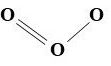
It is very reactive, which can be understood to mean that it has the tendency to readily interact with and alter things it contacts.
Where is it? We saw how it is a ground-level (i.e., tropospheric) secondary pollutant in the discussion of smog, but the focus of the current section is stratospheric ozone found high above the surface. The O3 molecules located between altitudes of about 10 and 50 kilometers[35] make up what is known as the ozone layer, although the name is a bit misleading because the gas is spread out within a large vertical column of the atmosphere. If consolidated at the surface, all the ozone molecules dispersed vertically within that 40-km column of atmosphere could be compressed to a width of just a few millimeters.
Cycle of formation and destruction. Existing O2 molecules produced from photosynthesis move to the stratosphere and are split into two single oxygen atoms. Each O then binds with another O2 molecule to form a total of two new O3. Ozone molecules can then be struck by ultraviolet radiation (UV) from the sun and split into a dioxygen molecule and a single O (a crucial reaction, as we will see). The cycle repeats indefinitely (Reaction 14.3.a and 14.3.b).
(Reaction 14.3.a) O2 → O + O then, for each O,
(Reaction 14.3.b) O + O2 → O3 → O2 + O
Uneven distribution. Complex global circulation patterns in the atmosphere lead to a dynamic and heterogeneous distribution of ozone. Research has revealed two important factors affecting O3 levels in the stratosphere.
Latitude
The amount of ozone in the stratosphere is not uniform around Earth. Simply put, movement due to prevailing winds leads to the highest O3 concentrations near the poles and lowest near the equator (Figure 14.28). It is a complicated story, though, because concentrations also vary with time (next paragraph).
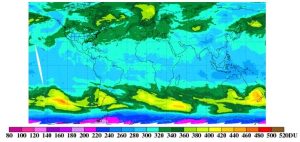
|
The Dobson Unit is used to measure ozone concentration in the atmosphere: 1 DU is equal to the number of molecules needed to make a layer of ozone that would be 0.01 mm thick at the Earth’s surface[36]. |
Time
In the short term, ozone levels fluctuate with season. Near Antarctica, for example, changes in temperature and other atmospheric properties combine to reduce O3 concentrations to their lowest points during September, October, and November, and then they rebound in December. The magnitude of these swings is dramatic, as levels rise or fall by one third or more from season to season. Changes are less pronounced at lower latitudes. In the long term, the 11-year sunspot cycle we encountered in the section on global warming contributes to variations in ozone concentration. Since O3 production is linked to UV-induced destruction of O2 molecules, average annual ozone levels tend to be at their maxima during times of highest solar energy output[37]. The challenge, then, is to detect changes in O3 concentration that exceed normal variations (i.e., are above background fluctuations).
Protective action of stratospheric ozone. Ozone in the stratosphere performs a critical service for the biosphere: it absorbs harmful incoming ultraviolet rays and prevents them from reaching Earth’s surface (Figure 14.29).
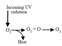
Note that when one of the O atoms is knocked off an ozone, yielding O2 and O, the UV energy that drove the reaction is converted to thermal energy. In other words, dangerous ultraviolet energy from the sun never makes it to ground level and instead heats the stratosphere. Why does this process matter? Without the ozone shield, life as we know it could not survive in terrestrial environments: intense UV energy would pass through the atmosphere and destroy the living cells it strikes (aquatic organisms living sufficiently deep would survive because water also absorbs UV). See Box 14.4 for more about the history and relevance of ozone in the stratosphere.
Box 14.4. Enjoying your ozone? (or: Box 1.1 reprised)
Remember Box 1.1? In a nutshell, it describes how our oxygenated atmosphere formed and why the earliest organisms were necessarily anaerobic. Here we can add that they were restricted to aquatic habitats because the lack of an ozone layer required those ancient creatures to live under water. Once photosynthesis developed, though, everything changed. We already know that the presence of dioxygen gas allowed for the evolution of aerobic organisms, but you should also realize that it led to the production and accumulation of O3 (via the processes described in Reaction 14.3). With the formation of the ozone layer, organisms did not need water to protect them from damaging UV and began to live on land. Once again we see the intimate connection between organisms and their environments!
Ozone depletion was noted decades ago.
The first hints were seen in the late 1950s and 1960s[38]. Using ground-based monitoring systems, researchers first recorded lower-than-expected levels of the gas near the South Pole in the winter of 1957. But the data were plagued by uncertainty and misunderstanding and deemed inconclusive at the time. Only in retrospect has the relevance of those early findings been recognized. During the 1960s and early 1970s, a few researchers hypothesized that certain anthropogenic compounds detected in the atmosphere, today broadly classified as ozone-depleting substances (ODS), could bring on the destruction of O3 molecules (more about these chemicals and their actions will be presented shortly).
Initial reactions by government, industry, and the public were hostile. Although based on models, limited sampling, and laboratory experiments, the early science was compelling enough to capture the attention of many with an interest in ODS. Manufacturers of the suspect compounds reacted antagonistically to the science while many people who used the compounds started to question if they were damaging Earth’s environments and endangering future generations. Political conflicts, advocacy on all sides, and worries about change, economic consequences, and inconvenience intensified[39]. The United States, home to a large fraction of producers and users of the controversial products, began to restrict certain applications of the compounds by the late 1970s even as research continued.
Science confirmed ozone loses in the 1980s[40]. During the 1980s, direct measurements over Antarctica verified what many already feared: the amount of ozone gas in the stratosphere was indeed decreasing. Even accounting for the background fluctuations described above, minimum concentrations of O3 dropped below 220 DU, the lowest level recorded prior to 1979 (and one assumed to result from anthropogenic influence on an otherwise natural cycle). Subsequent measurements revealed a continued decline into the early 2000s (Figure 14.30, top). At the same time, the size of the area of reduced O3 levels, the so-called ozone hole, got bigger and bigger (Figure 14.30, bottom).
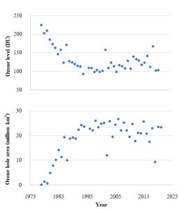
More about ozone-depleting substances
Although natural emissions—such as those from volcanoes—do play a minor role, research conducted in the 1980s strongly and clearly indicated that certain anthropogenic substances, two of which we will explore here, were responsible for most of the ozone depletion observed since the 1950s[41],[42].
Chlorofluorocarbons (CFCs). This large class of ODS will receive most of our attention due to the enormous role it plays in the depletion of ozone from the stratosphere. In an unrelated but important point, we saw compounds in this group previously because they are very powerful greenhouse gases.
Chemistry
Chlorofluorocarbons are built of various combinations of chlorine (Cl), fluorine (F), and carbon (C) atoms. Figure 14.31 shows two examples.
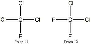
Applications
CFCs were once widely used as refrigerants in air conditioners and freezers, insulators, lubricants in engines, and aerosol propellants in cosmetics, medical devices, and paints[43]. The reason for this pervasiveness is straight forward: CFCs are both effective and non-reactive compounds. In other words, they not only perform their assigned tasks very well, they are unlikely to ignite or explode. This stability is clearly desirable in an appliance powered by electricity—for example, your refrigerator will not blow up if a spark accidently contacts the coolant gas. As we will see, new compounds have taken over the roles formerly carried out by CFCs, but historic emissions continue to influence stratospheric ozone.
How CFCs disrupt the natural equilibrium and contribute to ozone loss
Chemical stability. The same property that makes them so useful is also a big problem once they are released into the air. Unfortunately, they tend to persist in the troposphere because the conditions in the lower atmosphere are simply not conducive to their destruction. Residence time of individual CFCs varies, but some can remain in the troposphere for many decades.
Mobility, then breakdown. Complex circulation patterns in the atmosphere can carry CFCs up to the stratosphere. The intense ultraviolet radiation in this zone (unlike the conditions in the troposphere) separates them into their component chemicals, including extremely reactive chlorine atoms (the first “C” in the name “CFCs”). These freed Cl atoms, then, are responsible for the breakdown of O3 molecules. Reaction 14.4 shows one example of Cl-induced destruction of ozone.
(Reaction 14.4) 2O3 + Cl → 3O2 + Cl
Note the Cl atoms are called catalysts because they are not altered in the reaction—they only push ozone destruction forward and then are released, free to catalyze thousands of additional reactions until they are removed from the stratosphere by one of several slow, natural processes. The central idea here is that Cl atoms bring on a net loss of O3 molecules and a net increase in O2 within the stratosphere. Thus, the long-term natural equilibrium has been changed by human releases of chlorine-carrying gases such that ozone destruction outpaces ozone production (Figure 14.32)[44].
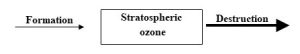
Bromine-containing gases. The element bromine (Br) is like chlorine in many important ways—both are halogens, a group of five elements with similar properties. Through a mechanism resembling the one described for chlorine, Br moves to the stratosphere and is released from the larger compounds in which it is a component. It then can catalyze the destruction of O3 molecules. For example, CBrClF2, a compound used in older fire extinguishers, once was an important source of reactive bromine atoms to the stratosphere. The pesticide methyl bromide (CH3Br), primarily used in agriculture, was another. Note that the previous sentences are written in the past tense because those compounds, like CFCs, have been largely phased out and replaced with substances that perform the same tasks but cause less ozone depletion (we will return to the topic of substitutes for ODS shortly).
Others. The chlorine and bromine gases described above, known as halogen source gases, make the largest anthropogenic contributions to O3 depletion. Swimming-pool disinfection, fossil fuel combustion, industrial processes, and other human activities can emit small amounts of depleting chemicals as well. Again, to minimize ozone damage, most of these processes now use different compounds.
The threat of ozone depletion
A net loss of O3 molecules from the stratosphere allows more harmful ultraviolet radiation to move to Earth’s surface and damage biological entities. Some models predict that, without appropriate corrective action, levels of UV would have reached high-enough levels to profoundly change the biosphere within a few decades. Here we consider some of the most important potential consequences.
Harm to human health.
Skin cancer
Skin cancers can be caused by the type of ultraviolet radiation absorbed by ozone[45]. Because more UV makes it to the surface with increasing destruction of stratospheric O3 molecules, higher rates of melanoma and other conditions are a concern. According to the United States Centers for Disease Control and Prevention (U.S. CDC), the rate of appearance of new skin cancers among Americans has increased in the past two decades, with the total number of new cases doubling between 1999 and 2019[46]. Now, many factors likely contribute to this observed trend, including changes in lifestyles, expectations, beach behavior, and so on, but loss of protective ozone during the same period is thought by many to play an important role.
Cataracts
This sight-limiting condition can be brought on by many agents, including exposure to ultraviolet radiation.
Immune disorders
Some evidence suggests UV radiation can alter immune function, increasing susceptibility to diseases. Further research must be done before definitive conclusions can be made about this consequence.
Harm to natural ecosystems.
Non-human organisms are also susceptible to UV-induced damage.
Effects on primary producers
Research has shown that terrestrial plants, even agricultural crops, can be adversely affected by ultraviolet radiation. As a result, organisms feeding directly or indirectly on these producers could also be harmed. Phytoplankton, aquatic primary producers, are similarly sensitive to increased UV levels because they live so close to the surface of water (and, therefore, are not deep enough to be protected). As we saw in our discussion of climate change, a loss in phytoplankton would devastate terrestrial and marine ecosystems.
Additional ecological effects
Organisms vary in their ability to tolerate exposure to ultraviolet radiation. High amounts of hair, fur, melanin, and various other structures provide some protection, so we would expect those having the appropriate adaptations to survive and reproduce more effectively than those that lack them. As we have seen throughout this textbook, ecosystem structure depends on environmental conditions, and we should expect that increasing amounts of UV reaching the surface to be like temperature, moisture, and all the others: it will influence the identity of dominant organisms throughout the biosphere. Eventually, if ozone levels were to drop sufficiently, terrestrial systems could become too hostile for any life forms—just as they were in the early days of this planet.
We have taken steps to restore ozone
Decades of research indicate that stratospheric-O3 concentration declined between the late 1960s and early 2000s. Moreover, although a few critics argued otherwise, the link between this loss and anthropogenic activity is strong. As emissions of ODS increased, the rate at which ozone was depleted became increasingly high relative to the rate at which it was produced. The chemical mechanism of ozone depletion was also understood. Clearly, this was a real phenomenon caused by humans, and corrective action was needed.
The Montreal Protocol: an international response. To combat the threat, 24 nations (plus the European Union) signed The Montreal Protocol on Substances that Deplete the Ozone Layer in 1987 (eventually, all UN members joined). Notably, signatories pledged to stop using CFCs and other O3-depleting compounds. The agreement evolved with time (and science), and many amendments were added during subsequent decades. The initial timeline for developed countries to phase out certain CFCs by the year 2000 (2010 for developing countries) was pushed forward to 1996, with some participants, including the United States, beating the deadlines.
Given the utility and widespread use of some of the ODS, adoption of the rules of the Protocol required a substantial commitment. Careful recycling and other steps were taken to reduce the release of existing chlorofluorocarbons into the air. Compounds that could substitute for CFCs without damaging ozone were also developed and slowly introduced into use (some of these are considered transitional because they only slow, rather than halt, O3 destruction and will themselves need to be replaced in the future). In the United States, for example, laws requiring non-ODS coolants in cars, refrigerators, and air conditioners were enacted during the 1990s. Other countries have taken similar steps.
Antarctic ozone levels have started to recover. It appears that the phasing out of ODS has allowed stratospheric ozone levels to slowly rebound. Recent measurements indicate O3 concentrations over Antarctica are rising. If the trends continue, the layer will recover to 1980s levels by the year 2065[47],[48]. We should proceed with caution, however. It is early in the process, O3 is still below its pre-1970 levels, and the long-lived ODS already in the troposphere will likely contribute to ozone destruction for decades. Also of concern is the possibility that CFCs or other problematic compounds could be released in the future by nations that either did not sign the Montreal Protocol or choose not to adhere to it. Be all that as it may, many people see the international response to the shared concern of ozone depletion, notably the cooperation among scientists, policy makers, governments, and members of the public, as a model that could be followed for future agreements about greenhouse gas emissions, global climate change, and other threats to the world.
14.2.5. More about reduction and regulation of outdoor air pollution
We end this section with a brief look at some of the strategies used to control air pollution.
Ways to limit emissions
Approaches to reduce the release of air pollutants generally fall into one of three categories: those that reduce emissions by increasing efficiency of energy-using technology, those that clean up pollutants before they move into the atmosphere, and those that rely on low- or no-pollution energy sources.
Increase efficiency. In this case, machines, vehicles, and appliances are designed to require less power to perform the same services we have always gotten from them. For example, televisions, refrigerators, and lights that provide entertainment, cold storage, and illumination, respectively, with less electricity than older models of the same devices lead to less burning of coal (a commonly used source of energy; see Chapter 10) and therefore lower levels of emissions than previously seen. Similarly, less gasoline is burned—meaning fewer pollutants are released—if more kilometers can be traveled per liter of fuel (i.e., miles per gallon).
Clean up emissions. Instead of improving efficiency, air pollutants can be broken down or otherwise captured before they reach the atmosphere. A common example of this strategy is the use of catalytic converters in automobiles. In short, exhaust passes through one of these devices—essentially, a small metal box—as it travels from the engine to the tailpipe (Figure 14.33).
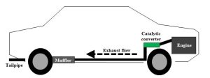
The converter contains metals like platinum and rhodium that speed up the conversion of certain pollutants produced from gasoline combustion, such as carbon monoxide and nitric oxide, into water and carbon dioxide (that is, the metals act as catalysts[49]). As part of the Federal Clean Air Act, the United States has mandated the use of catalytic converters on new cars for nearly 40 years, and many other countries have enacted similar laws. Arguably, this strategy has been successful in reducing certain types of local and regional air pollution, but it came with a very tangible price: converters add to the cost of a car. Emissions from coal-fired power plants can be reduced with analogous strategies, although in some cases the costs to install pollution controls are so high that affected companies choose to cease their use of coal in favor of cleaner fuels.
Use alternative energy sources. The combustion of non-renewable fossil fuels releases many more toxic products than does the use of renewables such as solar and wind power (Chapter 10). So, a third strategy is to replace conventional power generation technology, say, coal-burning electricity facilities, with something like wind farms. Phasing out carbon-based fuels in general would vastly reduce most of the adverse consequences of air pollution we have explored in this chapter. Chapter 10 describes several other benefits that a switch away from the dominant energy sources would bring, as well as the obstacles that have impeded wide-spread changes to alternative fuels.
How do we get polluters to make necessary changes?
Standards and expectations regarding air quality differ among countries, states, and localities. Effects of air pollution also vary, depending on local climate, environmental conditions, population density, and of course the specific substances of concern. As a result, regulations on anthropogenic air pollutants range in their scope, rigor, and underlying assumptions. Here we take a quick look at some commonly used approaches.
Direct regulation. In this case, governments pass laws that set emissions limits on all entities releasing a target pollutant. The catalytic converters we saw above fall into this category: they are required on every new car sold in the United States. Other sources, both mobile and stationary, can be controlled with direct regulation. In most cases, those that do not comply are punished with a fine.
Cap and trade. A second approach establishes a limit on the total amount of a pollutant released—that is, the cap—by a group of sources in a region. Then, individual members of this group buy the right or allowance to emit a certain amount of that substance each year. The total cap is lowered with passing years, compelling the entire class of polluters to reduce its emissions by whatever means it chooses (for example, using one or more of the three ways noted just above). Individual companies are incentivized to reduce their emissions as soon and as much as possible because, as less pollutant is released, fewer allowances are required. Moreover, those that have taken steps to innovate and clean up their emissions can sell their unneeded allowances to those that have not done as much to reduce pollutants. This market-based style of control provides far more flexibility than does direct regulation and is supported by many. Cap and trade was used to decrease the amount of sulfur dioxide released by coal-powered electricity generators in the United States during the 1990s, thereby reducing acid precipitation. The success of this effort to cut regional air pollution has inspired a movement to employ a similar model to lower carbon dioxide levels in the troposphere and combat global climate change. Not everybody is so ready to embrace such a policy, though, and debate about it has gone on for many years.
14.3. INDOOR AIR POLLUTION
Outdoor environments are not our only concern. People working and living in offices, schools, factories, laboratories, homes, and other interior areas can also be exposed to dangerous levels of airborne toxins. We close Chapter 14 with a few words about this serious public health problem.
14.3.1. A uniquely susceptible environment
Enclosed spaces are particularly vulnerable to air pollution by design (if not intention). To limit fluctuations in temperature and humidity without an undue financial cost, circulation with outside air is minimized. This situation can be understood through a familiar series of events: when air conditioning or heating is turned on, all doors and windows are tightly closed. So, any toxins present can become highly concentrated.
14.3.2. Many potential pollutants
As we saw with outdoor environments, the list of toxins here is long and diverse and includes chemical, physical, and biological entities. The possible adverse health outcomes caused by indoor air pollution also are quite numerous and varied.
Chemical
Chemical toxins come from many sources: solvents and adhesives, ozone from electrical appliances, fumes from newly painted walls or installed carpets, lead from old and peeling paint, insecticides used to control ants and the like, bathroom cleaners, cigarette smoke, perfumes, and many others. Depending upon the nature and degree of the odors these toxins emit, people may or may not know they are being exposed until symptoms appear. Responses vary, but burning of skin, eyes, or lungs, shortness of breath, nausea, blurred vision, light headedness, allergic reaction, asphyxiation, heart failure, and other outcomes are possible.
Physical
This category includes particulates like sawdust, asbestos fibers, fine mists, glass shards, and similar materials. These substances generally induce different responses than do chemical pollutants because they directly injure tissues. Asbestos, for example, can become embedded deep inside lungs and ultimately lead to cancer. Dusts and shards can cause serious abrasions throughout the respiratory system.
Biological
Viruses, pathogenic bacteria, and mold spores are the principle concerns here. As we learned in Chapter 3, the first two entities on the list can cause human diseases. If they become airborne and are adapted to survive long enough outside a human body, they can move among people and spread diseases like the common cold, COVID-19, influenza, pneumonia, and many others. Perhaps the most vivid example of this phenomenon is seen on commercial airplanes. If one passenger boards with a head cold, the virus that caused it may spread to anyone else inside the cabin who happens to breathe the same air (i.e., everybody). Not all present will necessarily get sick, but it is likely many will carry more than just their luggage when then exit the plane. Mold spores that cause allergic reactions, the final item on the list, are relevant in spaces that are dark and damp.
14.3.3. Mitigating indoor air pollution
Steps may be taken to reduce indoor air pollution. First, treatment and filtration systems installed inside air handlers can minimize the challenges caused by limited air circulation. Given the diverse nature of potential pollutants, though, coming up with remedies for all the potential problems can be complicated and costly. Second, biological entities can be at least partially controlled by changing the environmental conditions of spaces to discourage these unwanted organisms. Better lighting, repair of water leaks, installation of dehumidifiers, and application of chemical disinfectants are among the strategies used.
14.3.4. Some final considerations
Not all indoor spaces are affected by the same level of air pollution. A short list of the variables that account for the differences is presented here.
Year of construction
Since rules have changed with time, generally getting increasingly strict during the past several decades, the age of a building is a very important factor. For example, leaded paint and asbestos, two materials banned in the United States because of the adverse effects they have on human health, were both widely used until the 1970s. In other words, older buildings will likely face different problems than newer ones.
Location, design, and materials used
Regardless of age, certain buildings are just more prone to indoor air pollution than others. Certainly, damp and dark regions will likely be characterized by more mold problems than dry and sunny ones. Also very important, though, are the decisions made before, during, and after construction. If costs are cut on quality of materials, expertise of contractors, maintenance, and appropriateness of infrastructure, including air handling systems, users and residents of buildings could experience long-term exposure to toxic substances in their homes or workplaces. In some cases, illnesses affect multiple people occupying the same space, for example employees housed in a single complex. This phenomenon, often called sick-building syndrome, can create a great deal of protracted suffering and conflict because owners / operators of suspect spaces are generally loathe to admit deficiencies in air quality (and subsequently pay the high costs required to fix the problem), often dismissing claims that workplace exposure is responsible for observed adverse consequences. Indeed, it can be very difficult for scientists and regulators to establish a causative relationship between symptoms and careless, irresponsible, or even criminal actions made by those responsible for a building. We will more fully explore the effects of several common toxins on human health in the final chapter in this book.
THE CHAPTER ESSENCE IN BRIEF [50]
Many human activities release pollutants into the atmosphere. Fossil fuel combustion is of particular concern, as it contributes to multiple local-, regional-, and global-scale effects. Much scientific evidence has linked human activity to one critical effect in particular, the warming of Earth’s troposphere and consequent climate change. Stopping or even reversing the observed changes is difficult for multiple reasons, but reticence about switching away from carbon-dioxide-emitting power generation is among the biggest obstacles.
Think about it some more…[51]
In what ways are air pollution and water pollution similar? Different?
Can the same source of pollution contribute to local-, regional-, and global-scale concerns? How?
Carbon dioxide is a natural product (review Chapter 4, for example). Is it appropriate to categorize it as an air pollutant? Why or why not?
Drawing on the principle of environmental unity once again, connect the dots between melting arctic ice and low fuel efficiency in passenger cars (you might want to consult Chapter 10 as you ponder your answer). Here is another one: think about the way increasing standards of living worldwide (Chapter 8) could increase the amount of material in landfills…and ultimately lead to higher average global temperatures.
Are forests sources or sinks of carbon dioxide? Think back to Chapter 12 as you ponder your answer.
Why are the data-based connections between human activity and climate change so hard for some people to acknowledge? Arguably, denial of evidence has become more adamant in recent years, even as the science has become increasingly compelling and clear. What is going on? Can you think of any way to reach those folks who cannot accept the reality of human-driven climate change?
How can ozone gas be classified as an air pollutant in one instance and a necessary component of the atmosphere in another?
- NASA 2022. Global climate change, vital signs of the planet. www.ncei.noaa.gov/news/global-climate-202112 AND Climate.gov. 2022. www.climate.gov/news-features/understanding-climate/climate-change-global-temperature ↵
- National Oceanographic and Atmospheric Administration (NOAA). 2023. www.noaa.gov/news/2022-was-worlds-6th-warmest-year-on-record ↵
- 2024. World Meteorological Organization (WMO) ↵
- https://climatereanalyzer.org/clim/t2_daily/ ↵
- NASA 2022. Global climate change, vital signs of the planet. www.ncei.noaa.gov/news/global-climate-202112 AND Climate.gov. 2022. www.climate.gov/news-features/understanding-climate/climate-change-global-temperature ↵
- NASA. 2022. Is the Sun causing global warming?. climate.nasa.gov/faq/14/is-the-sun-causing-global-warming/ ↵
- NASA. 2001. Global Effects of Mount Pinutubo. earthobservatory.nasa.gov/images/1510/global-effects-of-mount-pinatubo ↵
- NASA. 2014. Measuring Earth's Albedo. earthobservatory.nasa.gov/images/84499/measuring-earths-albedo ↵
- NASA. What is the greenhouse effect? climate.nasa.gov/faq/19/what-is-the-greenhouse-effect/#:~:text=Credit%3A%20NASA%20Jet%20Propulsion%20Laboratory,it%20would%20be%20without%20them. ↵
- Climate.gov. Happy 200th birthday to Eunice Foote, hidden climate science pioneer www.climate.gov/news-features/features/happy-200th-birthday-eunice-foote-hidden-climate-science-pioneer ↵
- Anderson, Hawkins, Jones. 2016. CO2, the greenhouse effect and global warming: from the pioneering work of Arrhenius and Callendar to today's Earth System Models. Endeavour 40: 178-187. ↵
- U.S. Environmental Protection Agency (EPA). Global greenhouse gas emissions data. www.epa.gov/ghgemissions/global-greenhouse-gas-emissions-data ↵
- U.S. Environmental Protection Agency (EPA). Global greenhouse gas emissions data. www.epa.gov/ghgemissions/global-greenhouse-gas-emissions-data ↵
- National Oceanographic and Atmospheric Administration (NOAA). Increase in atmospheric methane set another record in 2021. www.noaa.gov/news-release/increase-in-atmospheric-methane-set-another-record-during-2021 ↵
- U.S. Environmental Protection Agency (EPA). Global greenhouse gas emissions data. www.epa.gov/ghgemissions/global-greenhouse-gas-emissions-data ↵
- U.S. Environmental Protection Agency (EPA). Global greenhouse gas emissions data. www.epa.gov/ghgemissions/global-greenhouse-gas-emissions-data ↵
- U.S. Environmental Protection Agency (EPA). Climate Change Indicators: US and Global Precipitation. www.epa.gov/climate-indicators/climate-change-indicators-us-and-global-precipitation#:~:text=Since%201901%2C%20global%20precipitation%20has,increases%20in%20precipitation%20than%20others.. ↵
- National Oceanographic and Atmospheric Administration (NOAA). Climate Change: Global Sea Level. www.climate.gov/news-features/understanding-climate/climate-change-global-sea-level#:~:text=April%2019%2C%202022-,Highlights,3.8%20inches)%20above%201993%20levels. ↵
- United Nations (UN). The Ocean Conference. www.un.org/sustainabledevelopment/wp-content/uploads/2017/05/Ocean-fact-sheet-package.pdf ↵
- National Oceanographic and Atmospheric Administration (NOAA). Climate Change: Global Sea Level. www.climate.gov/news-features/understanding-climate/climate-change-global-sea-level#:~:text=April%2019%2C%202022-,Highlights,3.8%20inches)%20above%201993%20levels. ↵
- It's hard to picture how much that is! 1 Gt of water occupies 1 cubic kilometer of space—a cube that is 1 km or 0.6 miles long in each dimension. ↵
- NASA. Global Climate Change. Vital Signs. climate.nasa.gov/vital-signs/ice-sheets/ ↵
- US Geological Survey (USGS). Where are Earth's glaciers located? www.usgs.gov/faqs/where-are-earths-glaciers-located ↵
- NASA. Global Climate Changes. Vital Signs. Greenland, Antarctica Melting Six Times Faster Than in the 1990s. climate.nasa.gov/news/2958/greenland-antarctica-melting-six-times-faster-than-in-the-1990s/#:~:text=Andrew%20Shepherd%20at%20the%20University,the%202010s—a%20sixfold%20increase. ↵
- National Oceanographic and Atmospheric Administration (NOAA). 2018. What is Ocean Acidification? PMEL carbon program. www.pmel.noaa.gov/co2/story/What+is+Ocean+Acidification%3F ↵
- [footnote]National Oceanographic and Atmospheric Administration (NOAA). 2018. What is Ocean Acidification? PMEL carbon program. www.pmel.noaa.gov/co2/story/What+is+Ocean+Acidification%3F ↵
- NASA. Earth Observatory. Phytoplankton Productivity Down in Gulf of Maine. earthobservatory.nasa.gov/images/149915/phytoplankton-productivity-down-in-gulf-of-maine#:~:text=Research%20published%20in%202021%20showed,warming%20has%20affected%20the%20phytoplankton ↵
- International Energy Agency (IEA). Carbon Capture, Utlisation and Storage. www.iea.org/fuels-and-technologies/carbon-capture-utilisation-and-storage ↵
- weather.gov/mob/katrina ↵
- United Nations (UN). The Ocean Conference. www.un.org/sustainabledevelopment/wp-content/uploads/2017/05/Ocean-fact-sheet-package.pdf ↵
- The Intergovernmental Panel on Climate Change. http://www.ipcc.ch ↵
- U.N Climate Change. http://unfccc.int ↵
- NASA. Do scientists agree on climate change? climate.nasa.gov/faq/17/do-scientists-agree-on-climate-change/Climate.NASA.gov ↵
- Written with contributions from Jeff Fetzer, NASA scientist. 2010. ClimateNASA.gov ↵
- National Oceanographic and Atmospheric Administration (NOAA). Stratospheric Ozone, Monitoring and Research in NOAA. www.ozonelayer.noaa.gov ↵
- esrl.noaa.gov/csd/assessments/ozone/2006/chapters/Q9.pdf ↵
- National Oceanographic and Atmospheric Administration (NOAA). Twenty Questions. esrl.noaa.gov/csd/assessments/ozone/2006/chapters/Q9.pdf ↵
- NASA Ozone Watch. esrl.noaa.gov/csd/assessments/ozone/2006/chapters/Q9.pdf ↵
- Perhaps this story sounds familiar? Does it remind you of the current debate about and denial of climate change science? ↵
- NASA Ozone Watch. esrl.noaa.gov/csd/assessments/ozone/2006/chapters/Q9.pdf ↵
- NASA Ozone Watch. esrl.noaa.gov/csd/assessments/ozone/2006/chapters/Q9.pdf ↵
- NASA Earth Observatory. earthobservatory.nasa.gov/world-of-change/Ozone ↵
- National Oceanographic and Atmospheric Administration (NOAA). Global Monitoring Laboratory. Chlorofluorocarbons (CFCs). gml.noaa.gov/hats/publictn/elkins/cfcs.html#:~:text=After%20World%20War%20II%2C%20CFCs,%2C%20homes%2C%20and%20office%20buildings. ↵
- National Oceanographic and Atmospheric Administration (NOAA). Twenty Questions. esrl.noaa.gov/csd/assessments/ozone/2006/chapters/Q9.pdf ↵
- U.S. Environmental Protection Agency. Ozone Layer Protection. www.epa.gov/ozone-layer-protection ↵
- U.S. Centers for Disease Control and Prevention (CDC). Melanoma of the Skin Statistics. www.cdc.gov/cancer/skin/statistics/index.htm ↵
- United Nations Environment Programme. Scientific Assessment of Ozone Depletion: 2022. Montreal Protocol on Ozone Depleting Substances quadrennial assessment report. ozone.unep.org/system/files/documents/Scientific-Assessment-of-Ozone-Depletion-2022-Executive-Summary.pdf ↵
- National Oceanographic and Atmospheric Administration (NOAA). Path to recovery of ozone layer passes significant milestone. research.noaa.gov/article/ArtMID/587/ArticleID/2900/Path-to-recovery-of-ozone-layer-passes-a-significant-milestone ↵
- US Energy Information Administration. Gasoline explained. eia.gov ↵
- As you will find throughout this book, here is very succinct summary of the major themes and conclusions of Chapter 14 distilled down to a few sentences and fit to be printed on a t-shirt or posted to social media. ↵
- These questions should not be viewed as an exhaustive review of this chapter; rather, they are intended to provide a starting point for you to contemplate and synthesize some important ideas you have learned so far. ↵
One of Earth's four spheres, this one contains all of Earth's water. See Chapter 4 for more.
One of Earth's four spheres, refers to all living things. See Chapter 4 for more.
One of Earth's four sphere. This term refers to the brittle, outer layer of the Earth made up of the entire crust and the upper portion of the mantle. It is nonliving and lies on top of the asthenosphere. See Chapter 3 for more.
An adjective that refers to organisms that live primarily on land (i.e., not in water). Compare to aquatic organisms. See Chapter 4 for more.
An adjective that refers to organisms that live in water. Compare to terrestrial. See Chapter 4 for more.
A gas made up of one carbon atom and two oxygen atoms, it is one of the many forms carbon can take. This gas is the product of aerobic respiration as well as combustion of fossil fuels, wood, and other materials containing organic carbon. It is not directly usable as a carbon source but can be fixed into useable forms of carbon, for example glucose, by autotrophic organisms. See Chapters 4 and 14 for more.
An adjective referring to an organism that uses dioxygen in its metabolism. "Aerobe" is the noun, the organism itself. Contrast with anaerobic. See Chapter 1 for more.
A general word that refers to the breaking down of relatively large, complex materials into relatively small, simple materials. Certain organisms, known as decomposers, break down the remains and waste products of other organisms and use those products as nutrient sources. Decomposers are critical to the health of ecosystems because they aid in the recycling of materials. Fungi and some bacteria are important decomposers. See Chapters 4 and 5 for more.
An adjective that means of human origin. See Chapter 7 for details.
A general chemical term that refers to chemical compounds made up of hydrogen and carbon atoms bonded together. This term encompasses a large array of compounds with different numbers of C and H atoms connected in different ways. See Chapter 10 for details and context.
A governing rule in environmental science that states, in short: all systems are connected to all other systems. The principle of environmental unity also implies that changes made to any system can bring about changes to other systems, even if those other systems are very distant from the initial change. Importantly, the resultant changes can be hard to predict and often are undesirable. See Chapter 1 for more.
In chemistry, occurs when two or more atoms are brought close together and interact. Reactions can lead to breaking of existing bonds and formation of new bonds. In some cases, separate smaller units are combined into larger units via reactions. Energy released during some reactions can be captured by organisms and used to do the work of living. See Chapter 4 for more.
An example of a very close mutualistic relationship involving algae and fungi. This association is so evolved and so close that lichens take on a form that is distinct from that of each partner. See Chapter 5 for details,
In chemistry, when a neutral atom gains or loses electrons, thereby gaining or losing negative charge, it becomes a charged ion. Loss of electrons produces a positive ion, gain of electrons produces a negative ion. See Chapter 4 for more.
In ecology, refers to the specific identity of organisms present in an ecosystem. This property varies widely among ecosystems. See Chapter 5 for details.
One of the processes carried out by organisms in an ecosystem. Important functions include C fixation, decomposition, and consumption. See Chapter 5 for details.
Often shortened to bioavailability. Refers to how ready accessible a substance is to organisms. High bioavailability is good for nutrients but can be harmful if the substance in question is toxic.
Organisms that fix carbon for all members of an ecosystem; they are autotrophs. They also tend to convert non-biologically available energy into biologically available forms. For example, plants both fix carbon and convert the sun's energy to chemical bond energy. Consumers live off of the C and energy stored in primary producers. See Chapters 4 and 5 for more.
A chemical substance released into the atmosphere that is converted into an acid. For example, sulfur dioxide gas emitted in coal combustion will react to form sulfuric acid. See Chapter 14 for more.
The amount of solar radiation reflected off any planetary body. See Chapters 4 and 14 for details.
Aerosol is a general term referring to any fine particle or droplet suspended in air.
The inner-most layer of the atmosphere, this is where weather events occur and is the portion of the atmosphere that is in direct contact with Earth's surface and living things. See Chapters 4 and 14 for more.
A pathway of the hydrologic cycle. Water changes from liquid to gas. See Chapter 4 for more.
A pathway of the hydrologic cycle. Water is drawn into plants via their roots. The water moves upwards and is released through openings in leaves as a vapor. See Chapter 4 for more.
In a system, current output accentuates or magnifies the effect of previous output. This type of feedback leads to change away from initial conditions. Compare to negative feedback. See Chapter 2 for more.
A process carried out by living things. The chemical bonds in relatively large molecules are broken with the following results: some energy is harnessed by the respiring organism and the large molecule is broken down into relatively small fragments. See Chapter 4 for more.
In chemistry, an adjective that refers to chemical compounds that consist of at least one C atom that is bonded to at least one H atom. Compare to inorganic. See Chapter 4 for details.
Formed from the remains of ancient organisms. These include coal, oil, and natural gas. They contain a lot of organic carbon compounds that are converted to inorganic products like CO2 when the fuels are burned. See Chapters 3 and 10 for details.
The human practice of cultivating crops and growing animals to produce food for human consumption. It involves extensive manipulations of natural environments and ecological processes. See Chapter 9 for details.
The removal of forest ecosystems. Multiple forces, anthropogenic and natural, can cause deforestation. See Chapter 12 for details.
A general term related to biogeochemical cycles. It refers to any process that increases the biological availability of an atom. See Chapter 4 for details.
A form of carbon that is biologically available to the whole biosphere. It is organic, having the formula C6H12O6. It is produced by fixation of carbon dioxide.
A group of organisms that are eukaryotic, phototrophic, and autotrophic. Some are unicellular, but most are colonial. Note: some scientists include certain prokaryotic cells in this group, the so-called "blue-green algae"; others classify those prokaryotic organisms as bacteria (known as "cyanobacteria"). We will follow the latter convention in this book. See Chapter 3 for more.
Refers to the many different kinds of microscopic organisms that are single celled and prokaryotic (i.e., do not possess distinct cellular organelles). Collectively, bacteria are extremely diverse, are the oldest organisms on Earth, and are critical to many environmental cycles and processes. See Chapter 3 for more.
More formally, 'aerobic organisms', they require dioxygen gas for survival. See Chapter 1, especially Box 1.1, for more.
Natural materials that are produced from chemical, biological, and physical transformations of rocks and organisms. True soil consists of layers or soil horizons. Soils consist of inorganic and organic materials + air and water. See Chapter 9 for details.
The movement of a material that is unequally spread throughout some medium (e.g., air or water) from areas of high concentration of the material to areas of low concentration of the material. See Chapter 4 for details.
A large mass of ice that persists for many years (up to hundreds of thousands) despite changing seasons. It is formed through accumulation and compression of snow into ice. Glaciers can profoundly shape the surface as they slowly move, store a lot of freshwater, and contain clues about past climatic and atmospheric conditions. See Chapters 4 and 14 for more.
An adjective referring to organisms that do not use dioxygen as part of their metabolism. Many such organisms die in the presence of oxygen gas. "Anaerobe" is the noun. Compare to aerobic. See Chapter 1 for more.
In ecology, a relationship among organisms in which all participants benefit. See Chapter 5 for details.
A structure designed to contain waste. See chapter 13 for details.
See Global Warming Potential.
A process that leads to the complete disappearance of a species from Earth. See Chapter 6 for more.
Refers to the salt content of water.
Refers to replacement of water in the groundwater reservoir. Recharge is largely the result of precipitation followed by infiltration of water downward. Melting snow and ice at the surface can also contribute. See Chapter 4 for more.
A reservoir of the hydrologic cycle located below the Earth's surface. See Chapter 4 for details.
Plant-like plankton that are producers; they are consumed by zooplankton. They live in surface waters where sunlight is available. They tend to be on the order of a few millimeters or so in size. See Chapter 5 for more.
A general term that includes any disease-causing organism. Some bacteria, fungi, protozoa, and algae are on this list, as are many viruses. Certain worms and other larger organisms can act as pathogens as well. See Chapters 3 and 5 for more.
A group of organisms that are microscopic, eukaryotic, mobile (also known as "motile"), and usually heterotrophic. They are roughly ten times larger than bacteria; they also tend to prey on bacteria. See Chapter 3 for more.
An important component of soil. It is a complex material made up of the partially decomposed remains of organisms. It supplies nutrients to plants and helps retain moisture and soil structure. See Chapter 9 for details.
A strategy that would collect carbon dioxide gas generated from fossil fuel combustion before it moves to the atmosphere. The captured carbon would then be used in the manufacturing of plastics. It is an idea that is in early stages of development. See Chapter 14 for more.
The increase in forested area compared to the current situation. In other words, forests would encroach upon un-forested areas. See Chapter 12 for details.
Refers to nations that have relatively small amounts of technology, wealth, and infrastructure compared to the developed world. See Chapter 8 for details.
Refers to nations that have relatively large amounts of technology, wealth, and infrastructure compared to the developing world. See Chapter 8 for details.
In systems analysis, feedback is defined as a system's response to its own output. See negative and positive feedback. See Chapter 2 for more.
The process of converting C from non-biologically available forms to forms that can be used by organisms. Typically, carbon dioxide molecules are converted to glucose. C fixation is carried out by organisms that possess the proper machinery to do so: plants, algae, and some bacteria. Fixation is a general term that indicates an increase in the biological availability of any atom. See Chapter 4 for more details.
The one requirement for growth that is least abundant relative to demand for it. It is a concept and problem relevant for both natural and agricultural systems. See Chapter 9 for details.
The layer, or soil horizon, that contains the most soil organic matter (SOM). It is is at or close to the surface. This is the most fertile part of the soil profile and is where plants grow; when it is lost, the remaining horizons cannot support plants, including crops. See Chapter 9 for details.
A property of any scientific measurement, it represents the size of the error term for a measurement. Can be thought of as the range of possible answers to a question (often, from lowest to highest). May be expressed as a number, e.g., 5.0 +/- 0.5 which indicates an average value (or otherwise representative number) of 5 with a possible range of 4.5 to 5.5. It arises from random and systematic errors. See Chapter 2 for more.
An area in the stratosphere in which there is less ozone than is typical. See Chapter 14 for more.
An important consideration when scientists make measurements. Background levels refer to the normal condition of whatever variable is under consideration. For example, normal human body temperature is 37 degrees C (98.6 F). Put another way, background is 37 (i.e., not 0); we use a thermometer to determine if temperature is ABOVE background (say 39) when a person is sick. Background levels can affect measurements and interpretations of experimental results. This idea is specifically referenced in Chapter 14 but is relevant for all scientific measurements and ideas described in the book.
A type of radiation emitted from the sun that is invisible to the human eye; can damage living tissues and cells. See Chapter 14 for more.
A process carried out by certain organisms (plants, algae, and some bacteria) in which the energy of the sun is used to drive the fixation of carbon. See Chapters 4 and 5 for more details.
